
Vector databases - like Weaviate - use machine learning models to analyze data and calculate vector embeddings. The vector embeddings are stored together with the data in a database, and later are used to query the data.
In a nutshell, a vector embedding is an array of numbers, that is used to describe an object. For example, strawberries could have a vector [3, 0, 1] – more likely the array would be a lot longer than that.
Note, the meaning of each value in the array, depends on what machine learning model we use to generate them.
To judge how similar two objects are, we can compare their vector values, by using various distance metrics.
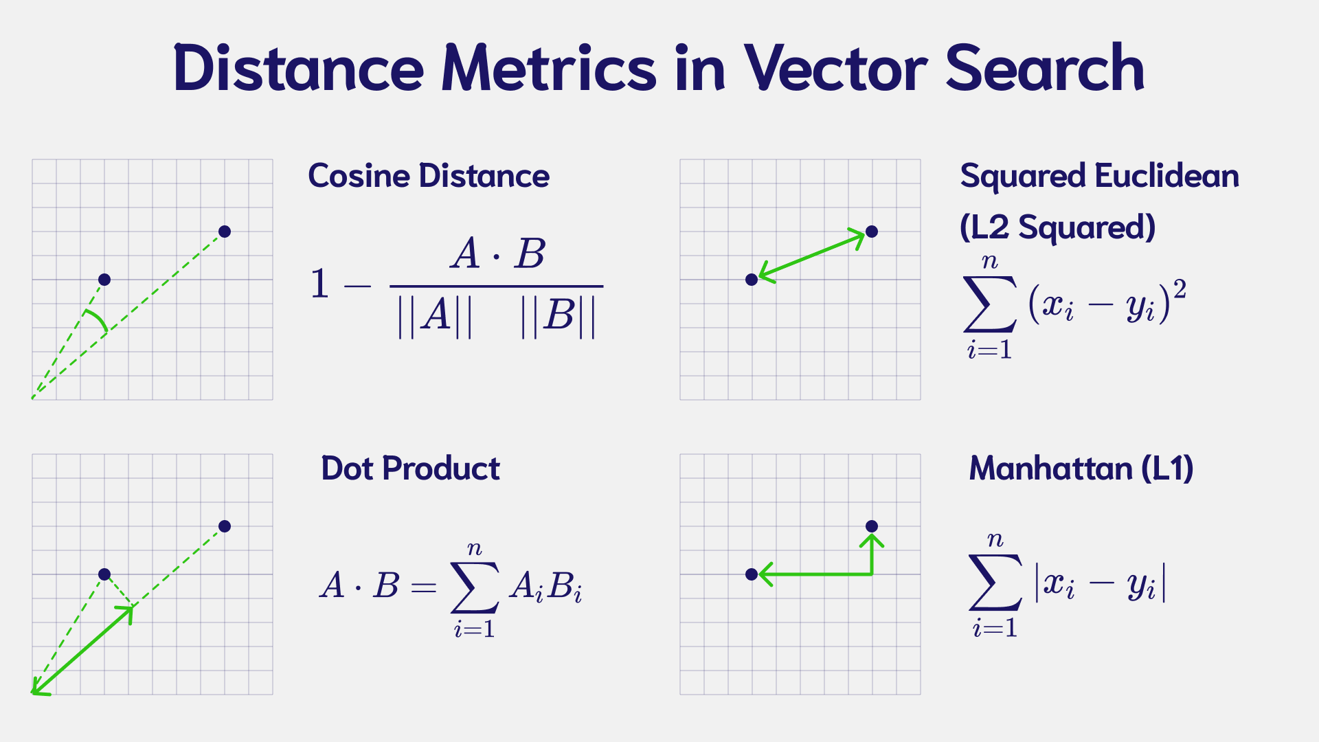
In the context of vector search, similarity measures are a function that takes two vectors as input and calculates a distance value between them. The distance can take many shapes, it can be the geometric distance between two points, it could be an angle between the vectors, it could be a count of vector component differences, etc. Ultimately, we use the calculated distance to judge how close or far apart two vector embeddings are. These metrics are used in machine learning for classification and clustering tasks, especially in semantic search.
Distance Metrics convey how similar or dissimilar two vector embeddings are.
In this article, we explore the variety of distance metrics, the idea behind each, how they are calculated, and how they compare to each other.
Fundamentals of Vector Search
If you already have a working knowledge of vector search, then you can skip straight to the Cosine Distance section.
Vectors in Multi-Dimensional Space
Vector databases keep the semantic meaning of your data by representing each object as a vector embedding. Each embedding is a point in a high-dimensional space. For example, the vector for bananas (both the text and the image) is located near apples and not cats.
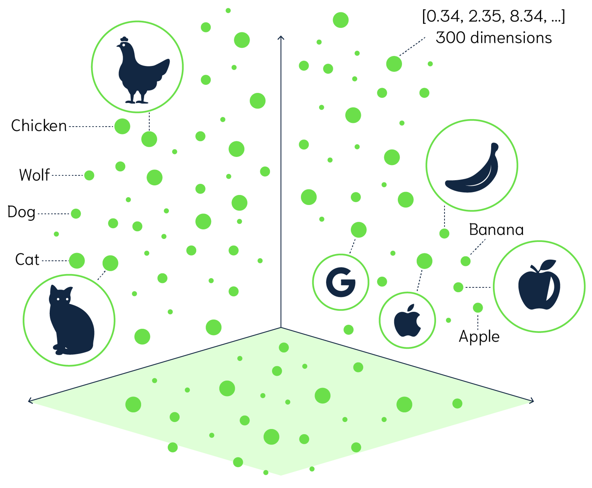
The above image is a visual representation of a vector space. To perform a search, your search query is converted to a vector - similar to your data vectors. The vector database then computes the similarity between the search query and the collection of data points in the vector space.
Vector Databases are Fast
The best thing is, vector databases can query large datasets, containing tens or hundreds of millions of objects and still respond to queries in a tiny fraction of a second.
Without getting too much into details, one of the big reasons why vector databases are so fast is because they use the Approximate Nearest Neighbor (ANN) algorithm to index data based on vectors. ANN algorithms organize indexes so that the vectors that are closely related are stored next to each other.
Check out this article to learn "Why is Vector Search are so Fast" and how vector databases work.
Why are there Different Distance Metrics?
Depending on the machine learning model used, vectors can have ~100 dimensions or go into thousands of dimensions.
The time it takes to calculate the distance between two vectors grows based on the number of vector dimensions. Furthermore, some similarity measures are more compute-heavy than others. That might be a challenge for calculating distances between vectors with thousands of dimensions.
For that reason, we have different distance metrics that balance the speed and accuracy of calculating distances between vectors.
Distance Metrics
Cosine Similarity
The cosine similarity measures the angle between two vectors in a multi-dimensional space – with the idea that similar vectors point in a similar direction. Cosine similarity is commonly used in Natural Language Processing (NLP). It measures the similarity between documents regardless of the magnitude.
This is advantageous because if two documents are far apart by the euclidean distance, the angle between them could still be small. For example, if the word ‘fruit' appears 30 times in one document and 10 in the other, that is a clear difference in magnitude, but the documents can still be similar if we only consider the angle. The smaller the angle is, the more similar the documents are.
The cosine similarity and cosine distance have an inverse relationship. As the distance between two vectors increases, the similarity will decrease. Likewise, if the distance decreases, then the similarity between the two vectors increases.
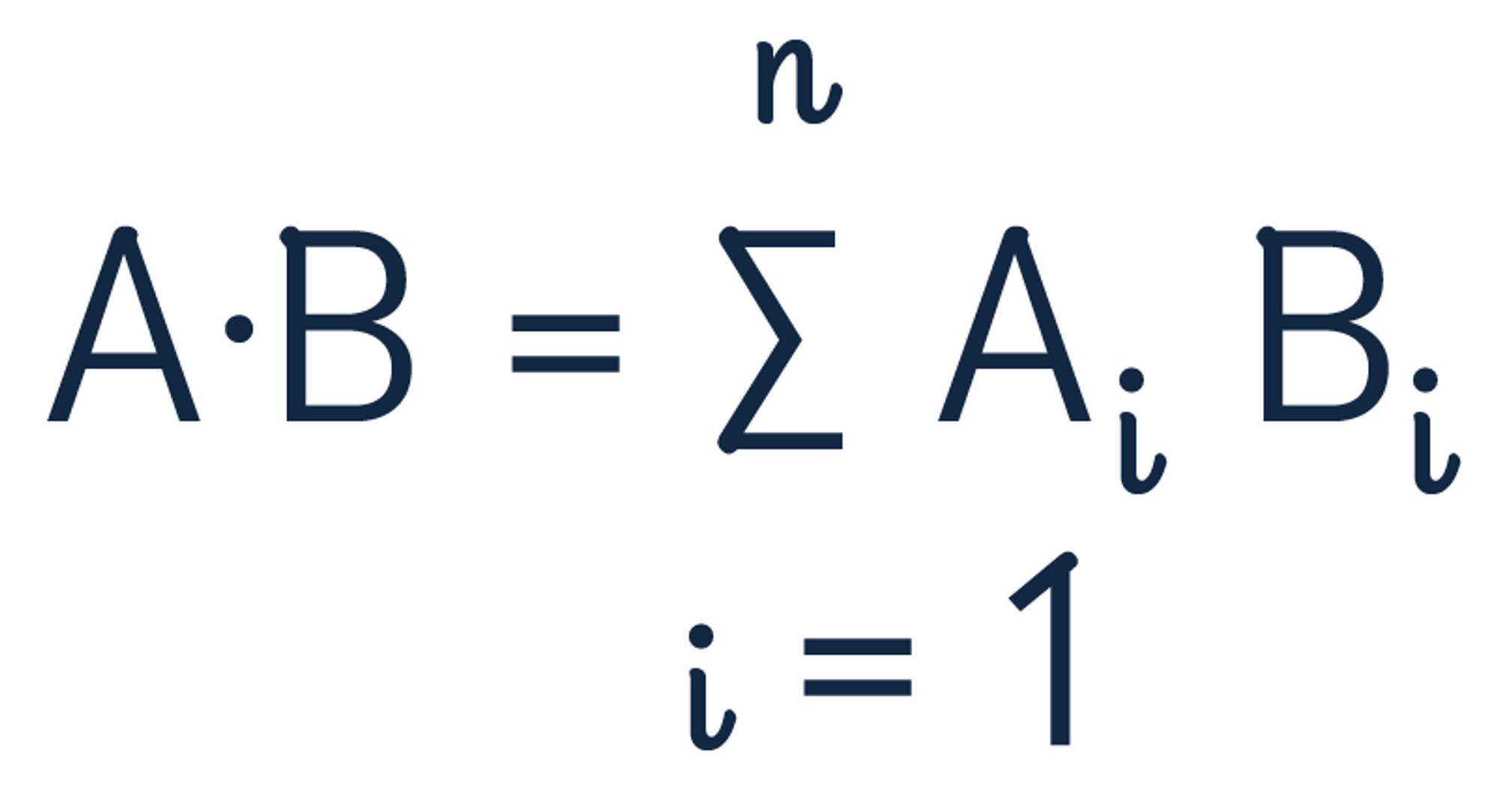
The cosine similarity is calculated as:
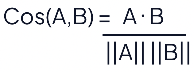
A·B is the product (dot) of the vectors A and B
||A|| and ||B|| is the length of the two vectors
||A|| * ||B|| is the cross product of the two vectors
The cosine distance formula is then: 1 - Cosine Similarity
Let's use an example to calculate the similarity between two fruits – strawberries (vector A) and blueberries (vector B). Since our data is already represented as a vector, we can calculate the distance.
Strawberry → [4, 0, 1]
Blueberry → [3, 0, 1]
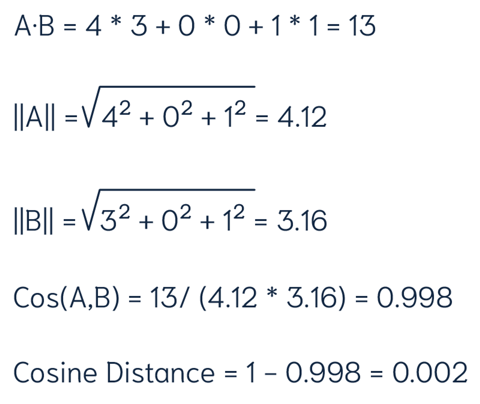
A distance of 0 indicates that the vectors are identical, whereas a distance of 2 represents opposite vectors. The similarity between the two vectors is 0.998 and the distance is 0.002. This means that strawberries and blueberries are closely related.
Dot Product
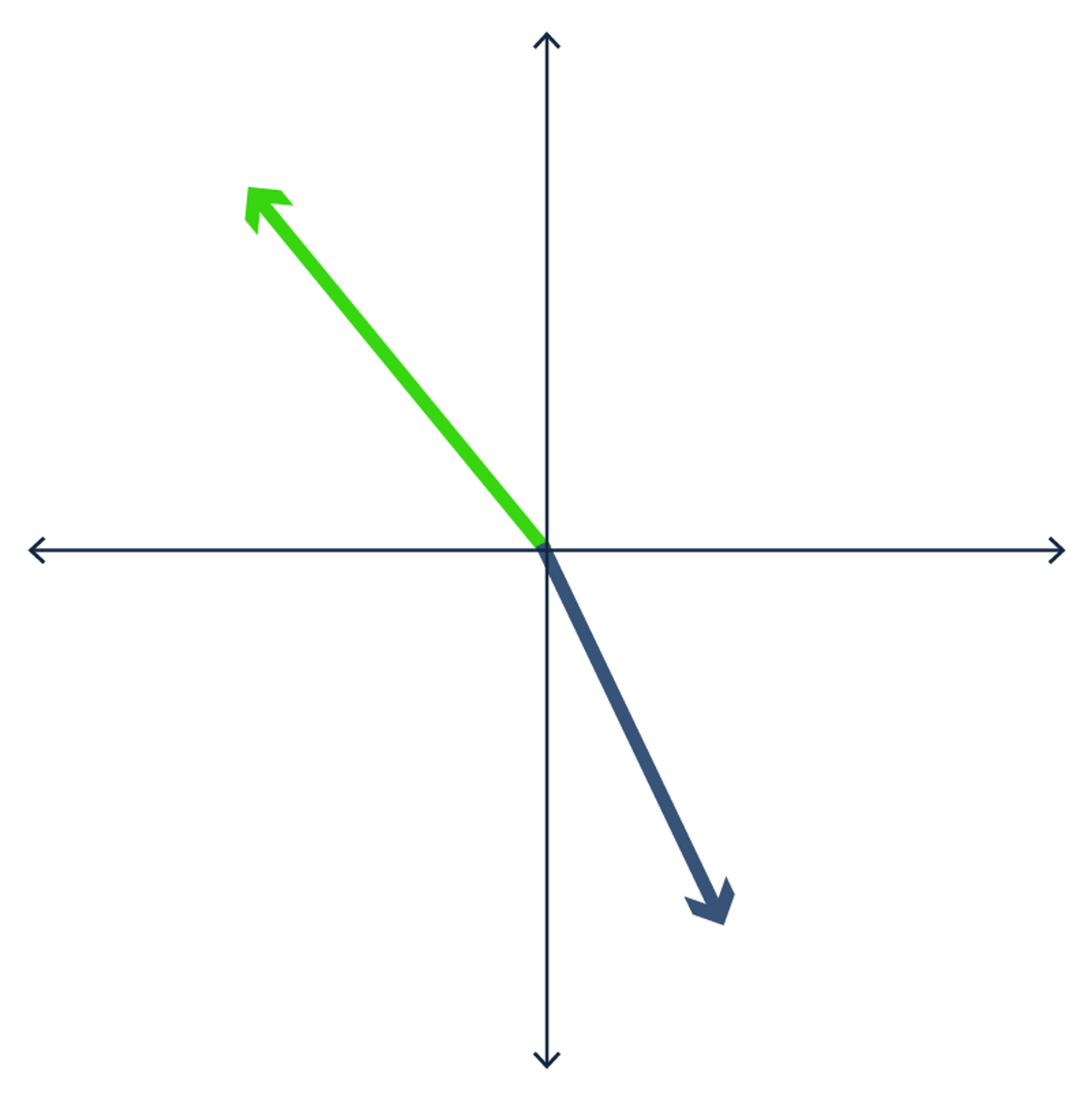
The dot product takes two or more vectors and multiplies them together. It is also known as the scalar product since the output is a single (scalar) value. The dot product shows the alignment of two vectors. The dot product is negative if the vectors are oriented in different directions and positive if the vectors are oriented in the same direction.
The dot product formula is:
Use the dot product to recalculate the distance between the two vectors.
Strawberry → [4, 0, 1]
Blueberry → [3, 0, 1]

The dot product of the two vectors is 13. To calculate the distance, find the negative of the dot product. The negative dot product, -13 in this case, reports the distance between the vectors. The negative dot product maintains the intuition that a shorter distance means the vectors are similar.
Squared Euclidean (L2-Squared)
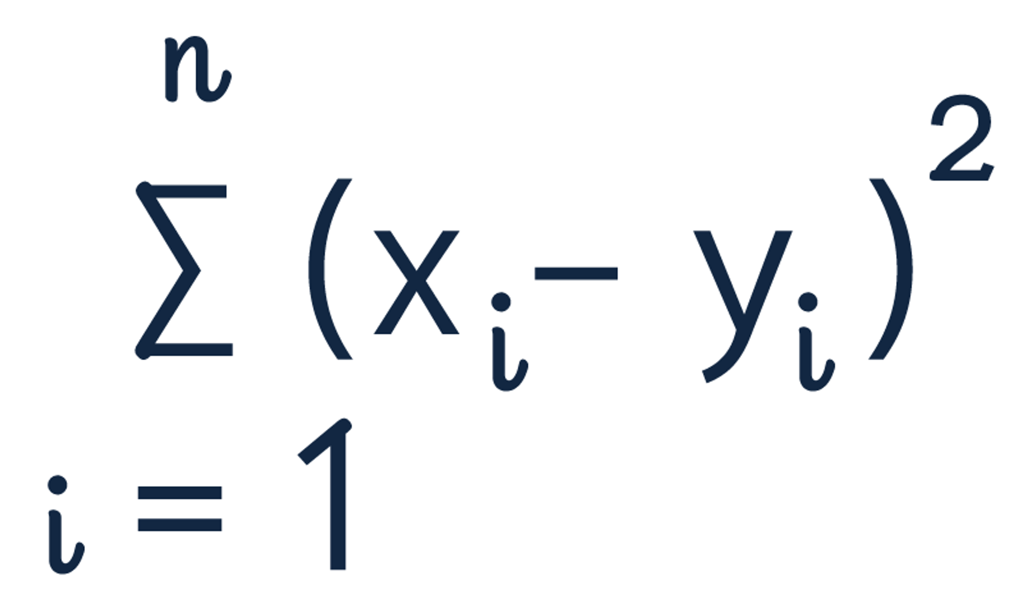
The Squared Euclidean (L2-Squared) calculates the distance between two vectors by taking the sum of the squared vector values. The distance can be any value between zero and infinity. If the distance is zero, the vectors are identical. The larger the distance, the farther apart the vectors are.
The squared euclidean distance formula is:
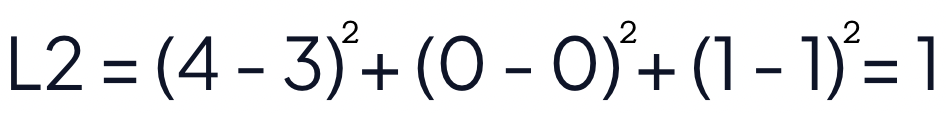
The squared euclidean distance of strawberries [4, 0, 1] and blueberries [3, 0, 1] is equal to 1.
Manhattan (L1 Norm or Taxicab Distance)
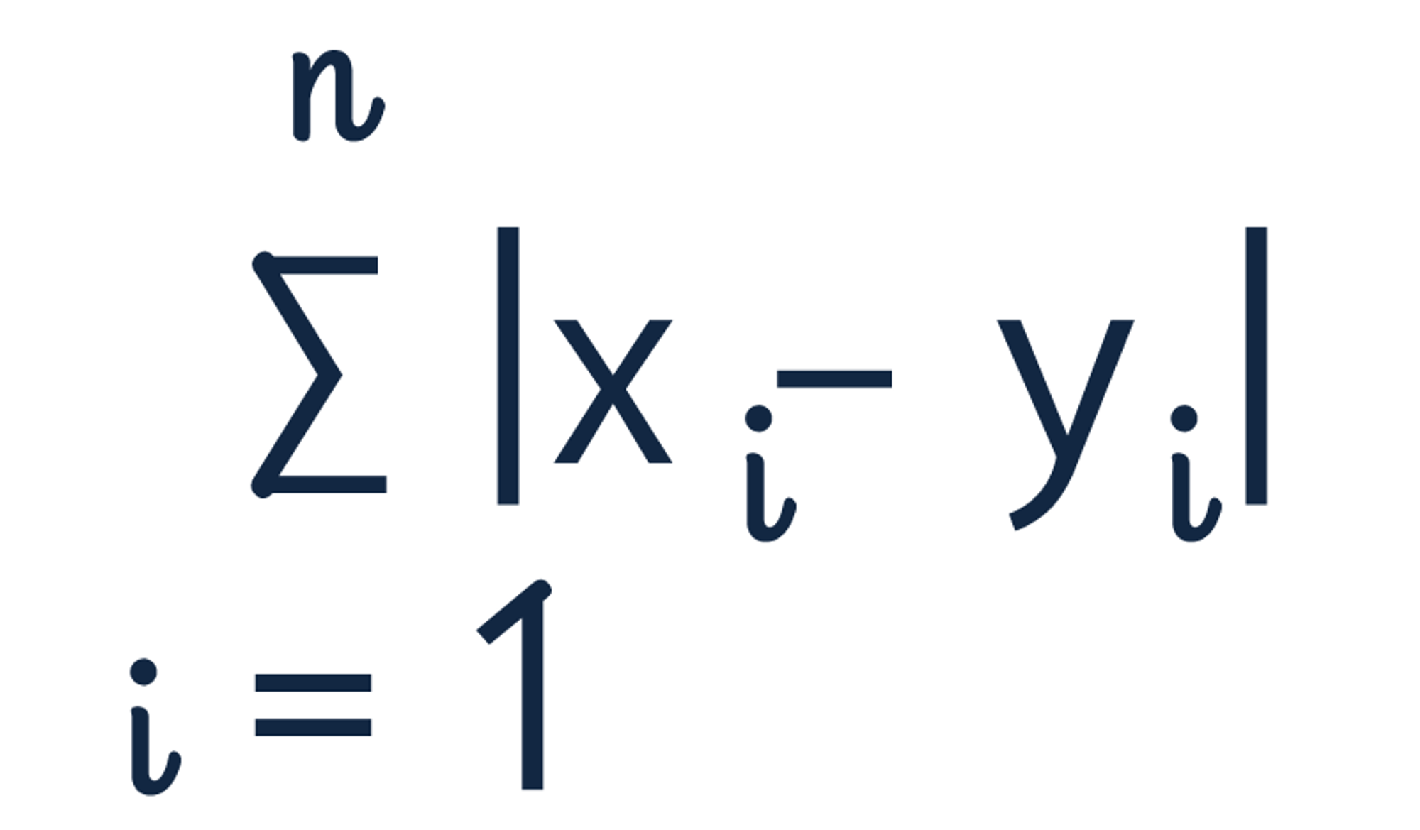
Manhattan distance, also known as "L1 norm" and "Taxicab Distance", calculates the distance between a pair of vectors. The metric is calculated by summing the absolute distance between the components of the two vectors.
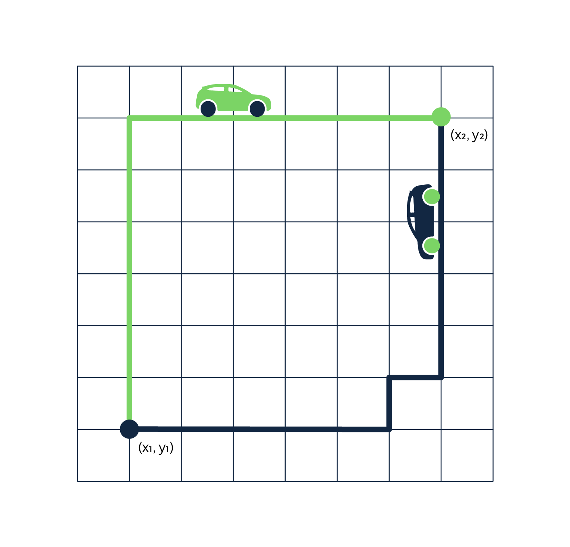
The name comes from the grid layout resembling the streets of Manhattan. The city is designed with buildings on every corner and one-way streets. If you're trying to go from point A to point B, the shortest path isn't straight through because you cannot drive through buildings. The fastest route is one with fewer twists and turns.
Hamming
The Hamming distance is a metric for comparing two numeric vectors. It computes how many changes are needed to convert one vector to the other. The fewer changes are required, the more similar the vectors.
There are two ways to implement the Hamming distance:
- Compare two numeric vectors
- Compare two binary vectors
Weaviate has implemented the first method, comparing numeric vectors. In the next section, I will describe an idea to use the Hamming distance in tandem with Binary Passage Retrieval.
Let's use an example to calculate the Hamming distance. Imagine we have a dataset containing a variety of fruit and vegetables. Your first query is to see which item pairs best with your banana pancakes. To achieve that we need to compare the banana pancakes' vector with the other vectors. Like this:
| Banana Pancakes | [5,6,8] | Hamming Distance |
|---|---|---|
| Blueberries | [5,6,9] | 1 |
| Broccoli | [8,2,9] | 3 |
As seen above, blueberries are a better pairing than broccoli. This was done by comparing the position of the numbers in the vector representations of foods.
Hamming distance and Binary Passage Retrieval
Binary Passage Retrieval (BPR) translates vectors into a binary sequence. For example, if you have text data that has been converted into a vector ("Hi there" -> [0.2618, 0.1175, 0.38, …]), it can then be translated to a string of binary numbers (0 or 1). Although it is condensing the information in the vector, this technique can keep the semantic structure despite representing it as 0 or 1.
To compute the Hamming distance between two strings, you compare the position of each bit in the sequence. This is done with an XOR bit operation. XOR stands for "exclusive or", meaning if the bits in the sequence do not match, then the output is 1. Keep in mind that the strings need to be of equal length to perform the comparison. Below is an example of comparing two binary sequences.
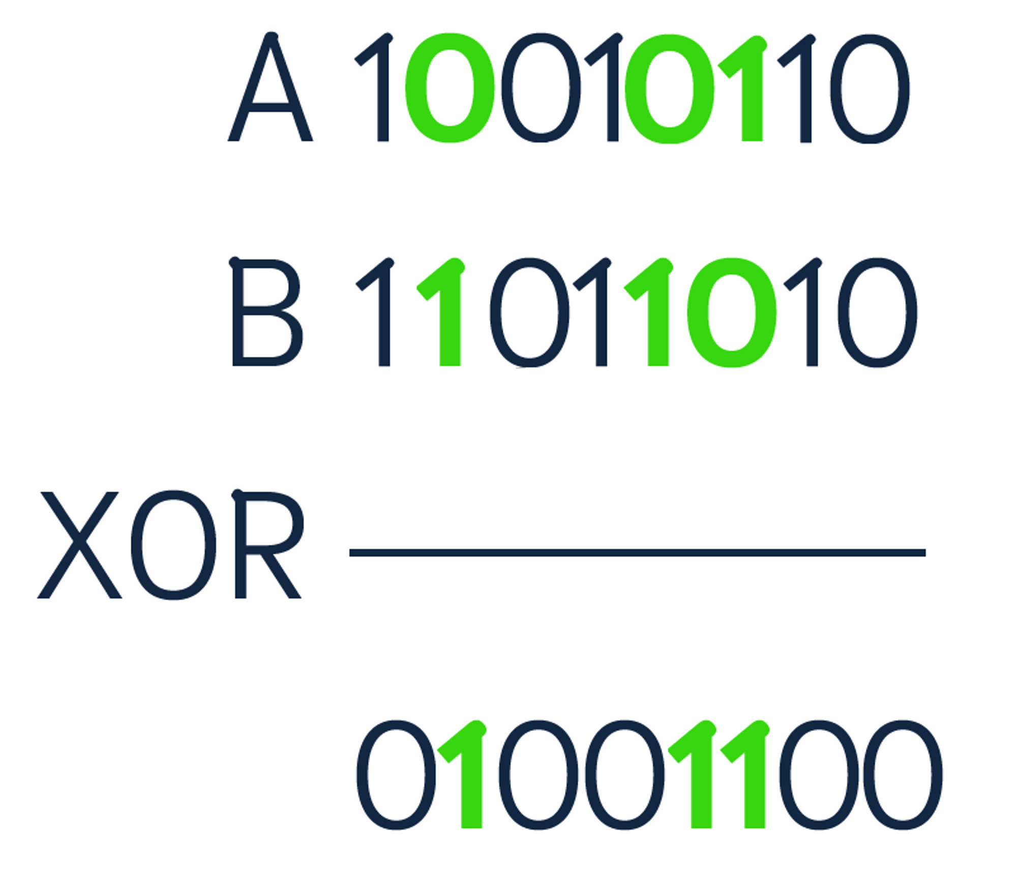
There are three positions where the numbers are different (highlighted above). Therefore, the Hamming distance is equal to 3. Norouzi et al. stated that binary sequences are storage efficient and allow storing massive datasets in memory.
Comparison of Different Distance Metrics
Cosine versus Dot Product
To calculate the cosine distance, you need to use the dot product. Likewise, the dot product uses the cosine distance to get the angle of the two vectors. You might wonder what the difference is between these two metrics. The cosine distance tells you the angle, whereas the dot product reports the angle and magnitude. If you normalize your data, the magnitude is no longer observable. Thus, if your data is normalized, the cosine and dot product metrics are exactly the same.
Manhattan versus Euclidean Distance
The Manhattan distance (L1 norm) and Euclidean distance (L2 norm) are two metrics used in machine learning models. The L1 norm is calculated by taking the sum of the absolute values of the vector. The L2 norm takes the square root of the sum of the squared vector values. The Manhattan distance is faster to calculate since the values are typically smaller than the Euclidean distance.
Generally, there is an accuracy vs. speed tradeoff when choosing between the Manhattan and Euclidean distance. It is hard to say precisely when the Manhattan distance will be more accurate than Euclidean; however, Manhattan is faster since you don't have to square the differences. You want to use the Manhattan distance as the dimension of your data increases. For more information on which distance metric to use in high-dimensional spaces, check out this paper by Aggarwal et al.
How to Choose a Distance Metric
As a rule of thumb, it is best to use the distance metric that matches the model that you're using. For example, if you're using a Siamese Neural Network (SNN) the contrastive loss function incorporates the euclidean distance. Similarly, when fine-tuning your sentence transformer you define the loss function. The CosineSimilarityLoss takes two embeddings and computes the similarity based on the cosine similarity.
To summarize, there is no ‘one size fits all' distance metric. It depends on your data, model, and application. As mentioned above, there are cases where the cosine distance and dot product are the same; however, the magnitude may or may not be important. This also goes for the accuracy/speed tradeoff between the Manhattan and euclidean distance.
Use the distance metric that matches the model that you're using.
Implementation of Distance Metrics in Weaviate
In total, Weaviate users can choose between five various distance metrics to support their dataset. In the Weaviate documentation you can find each metric in detail. Weaviate makes it easy to choose a metric depending on your application. With one edit to your schema, you can use any of the metrics implemented in Weaviate (cosine, dot, l2-squared, hamming, and manhattan), or you have the flexibility to create your own!
Distance Implementations and Optimizations
Even with ANN-indexes, which reduce the number of distance calculations necessary, a vector database still spends a large portion of its compute time calculating vector distances. As a result, it is very important that the engine can do this not just correctly, but also efficiently.
The distance metrics in Weaviate have been optimized to be highly efficient using "Single Instruction, Multiple Data" ("SIMD") instruction sets. Using these instructions, a CPU can do multiple calculations in a single CPU cycle. To achieve this, we had to write some of our distance metrics in pure Assembly code. Here is an overview of the current state of optimizations; including which distance metrics have SIMD optimizations for which architecture.
Open-source Contributions
Weaviate is open-source and values feedback and input from the community. A community member contributed to the Weaviate project by adding two new metrics to the 1.15 release. How cool is that! If this is something you're interested in, here is the repository with the implementation of the current metrics.
Ready to start building?
Check out the Quickstart tutorial, and begin building amazing apps with the free trial of Weaviate Cloud Services (WCS).