
The Tile Encoder - Exploring ANN algorithms Part 2.2
In our previous post, we explained how to compress vectors in memory. This was an important first step since we could still have a coarse representation of the vectors to guide our search through queries with a very low memory footprint. We introduced HNSW+PQ and explained the most popular encoding technique: KMeans, which can be used to find a compressed representation of vectors. While KMeans gives very good results, there are a couple of drawbacks. Firstly, it is expensive to fit to data. Secondly, when compressing vectors, it needs to calculate distances to all centroids for each segment. This results in long encoding and indexing times.
In this blog post, we present an alternative to KMeans, the Tile encoder, which is a distribution-based encoder. The Tile encoder works very similarly to KMeans but it doesn’t need to be fit to the data since it leverages the fact that we know the underlying distribution of the data beforehand.
Tile Encoder
KMeans produces a tiling over the full range of values using the centroids. Each centroid has a tile associated with it. When a new vector has to be encoded, the algorithm checks which tile it belongs to, and the vector code is set using the index of the closest found tile. When fitting KMeans to our data the generation of the tiles is not homogeneous. As a result, we expect more tiles where there is a higher density of data. This way the data will be balanced over the centroids.
Let’s take a moment to explore how the centroids that KMeans fits to our data are distributed. If we use one segment per dimension on Sift1M the centroids are distributed as shown in Figure 1.
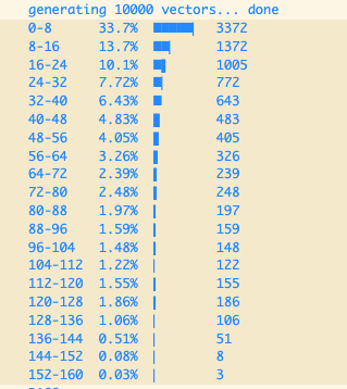
Fig. 1: Centroids distributions for the first dimension on Sift1M. Notice how the centroids are distributed with a LogNormal distribution centered at zero.
The centroids clearly follow a LogNormal distribution. This is a consequence of the dimension values following the same distribution. All dimensions in Sift1M and Gist1M are distributed with a LogNormal distribution. All dimensions in DeepImage96 follow a Normal distribution instead. The distribution of the data will be conditioned by the vectorizing method used to produce the vectors.
If we know the distribution of the data in advance, we might be able to produce the centroids without fitting the data with KMeans. All we need to do is to produce a tiling over the full range of values following the distribution of the data.
Let’s say we want to produce a byte code for each dimension. This would be similar to using KMeans with a dimension per segment. Instead of using KMeans, we could generate the codes using the Cumulative Density Function (CDF) of the distribution of the data. The CDF produces values from zero to one. We want 256 codes but in general we might want to use any amount of codes (so we could use more, or less bits to encode). The code then could be calculated as where is the amount of codes to use.
On the other hand, when we need to decompress the data, we need to generate the centroids from the codes. For this we need to use the inverse of the CDF function, meaning that we need the Quantile function. The real advantage of this approach is that we no longer need to spend a long time to fit our data. We could calculate the mean and standard deviation (only parameters of the distribution) incrementally as the data is added and that is it.
This also opens a good opportunity for easily updating the Product Quantization data over time since the whole process is very cheap in terms of time. This case would be interesting if for example we would have drifting data. If we compress the data and the data starts drifting due to some new trends, then the distribution of the data changes and the compression data (KMeans centroids and codes generated from them) will become outdated. With the Tile encoder we could monitor this situation and update data very quickly.
Centroid Distributions
To get a better understanding of the distribution of the centroids, let us create some illustrations with the generated centroids.

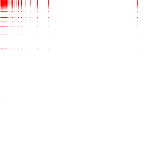
Fig. 2: Centroids generated by the KMeans and Tile encoders. Both charts show the cartesian product of the first two segments. Both encoders were fitted using 32 centroids. Above we show the centroids from KMeans. Below we show the centroids from Tile.
As we can observe. Both approaches generate similar results. The centroids are very dense at the origin of both axes and much more sparse as the values grow. It is worth mentioning that a multivariate approach would fit the data better than the cartesian product of individually built segments. To depict this, we show Figure 3.


Fig. 3: Centroids generated by KMeans on the first segment including the first two dimensions. The encoder was fitted using 32 (above) and 256 (below) centroids. Centroids fit better the distribution of the data as opposed to using independent segments for each dimension when using enough centroids.
We are yet to extend the tile encoder to the multivariate case. Although this is not extremely difficult it still needs some work and will be included in the near future. We have decided to publish this initial implementation so it can be tested with more data.
Notice that this encoder depends on the fact that the distribution of the data is known a priori. This means that you need to provide this information beforehand. Currently we support normal and lognormal distributions which are very common. If your data follows a different distribution, extending the code is very simple so do not hesitate to contact us.
Results of the KMeans Vs Tile encoding
In this section we present some results on the comparison of Product Quantization using KMeans vs the Tile encoder.
Table 1 shows a comparison of Product Quantization using KMeans and the Tile encoders. We compare the time to calculate distance, the time to fit and encode the data and the recall. We only compare it to KMeans with one dimension per segment since the tile encoder would only support this setting for now. Also, fitting and encoding times were run on 10 cores concurrently, while distance calculations are based on single core metrics.
| Database | Data size | Fit | Encode | Time to calculate distance () | Recall | |
|---|---|---|---|---|---|---|
| KMeans | Sift | 1 M | 3m15s | 1m30s | 701 | 0.9973 |
| Gist | 1 M | 22m52s | 10m10s | 5426 | 0.95 | |
| DeepImage96 | 1 M | 2m14s | 10m17s | 5276 | 0.9725 | |
| Tile | Sift | 1 M | 294ms | 2s | 737 | 0.9702 |
| Gist | 1 M | 4s | 16s | 5574 | 0.962 | |
| DeepImage96 | 9.99 M | 122ms | 8s | 5143 | 0.9676 |
Table 1: Results of Product Quantization using KMeans and Tile encoders.
The recall results above are positive. We have lower recall in Sift and DeepImage datasets with the Tile compared to the KMeans encoder. On Gist we actually have better recall results with the Tile compared to the KMeans encoder. The cause for this difference has not yet been identified at the moment of writing this post. One significant difference is the vector size. It could be that independent errors for off distribution points on single dimensions are less significant on larger vectors since they will be absorbed by the rest of the dimensions. This is just an assumption though.
The results in terms of performance are very positive. First notice that fitting and encoding run in ten cores concurrently. This means that if you would run it single threaded, fitting 200,000 vectors and encoding the whole data on Gist with KMeans would have taken nearly 5 hours. In contrast, with the Tile encoder it would be nearly three minutes.
Additionally, notice that when Product Quantization is used with HNSW, we will need to compress at some point. This will mean fitting the existing data and encoding existing vectors. It will also need to compress the rest of the incoming vectors as they come. When using KMeans, we will need to wait for a period of time when our data is being compressed. During this time, the server will not be able to serve queries, since data is not ready for use. With the Tile encoder, the compress action will return a ready state almost immediately.
Furthermore, we need some data to trigger the compress action since we need the encoder to learn the distribution of data. Compressing too soon could affect the precision of the encoding. Also, notice that the indexing process rests upon the search procedure. Querying time could be reduced or increased depending on the segmentation of your data. If you are aiming to preserve recall, then you will most likely not use a coarse segmentation, meaning the querying time will be increased rather than shortened. Longer querying times lead to longer indexing times. The sooner we compress, the longer the indexing time will be in this situation, since more data will be indexed under compressed settings. The later we compress, the longer it will take for the KMeans to fit since it will have more data to fit on. On the other hand, fitting with Tile will be almost immediate so the later we compress the faster the indexing. In fact, if you have enough memory to index your data uncompressed, but you only need to compress the data after it is indexed (because of some operational restrictions) then we suggest you index as normal, and then you compress your data using Tile encoder since then the indexing time will remain unchanged compared to regular HNSW. If you use KMeans though, there is no way to keep indexing time as short as regular HNSW.
Performance Results
In the following figures we show the performance of HNSW+PQ on the three databases scoped on this post. All experiments were performed adding 200,000 vectors using uncompressed behavior, then compressing and adding the rest of the data. As mentioned before, if you add all your data and then compress with the Tile encoder, you would obtain the same indexing time as you would have when using regular HNSW. If you do so, then at the end you will need less memory for querying your server but at the moment of indexing you would actually need more memory since at some point you would have all vectors uncompressed and compressed but you will free the uncompressed vectors right after indexing.
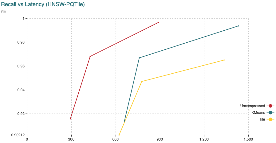 Fig. 4: *The chart shows Recall (vertical axis) Vs Latency (in microseconds, on the horizontal axis). For this experiment we have added 200,000 vectors using the normal HNSW algorithm, then we switched to compressed and added the remaining 800,000 vectors. *
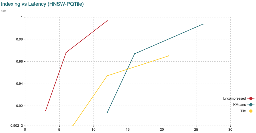 Fig. 5: The chart shows Recall (vertical axis) Vs Indexing time (in minutes, on the horizontal axis). For this experiment we have added 200,000 vectors using the normal HNSW algorithm, then we switched to compressed and added the remaining 800,000 vectors.
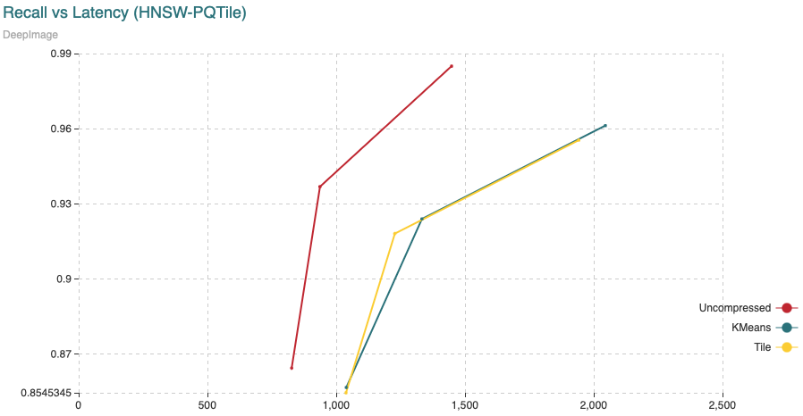 Fig. 6: The chart shows Recall (vertical axis) Vs Latency (in microseconds, on the horizontal axis). For this experiment we have added 1,000,000 vectors using the normal HNSW algorithm, then we switched to compressed and added the remaining 8,990,000 vectors.
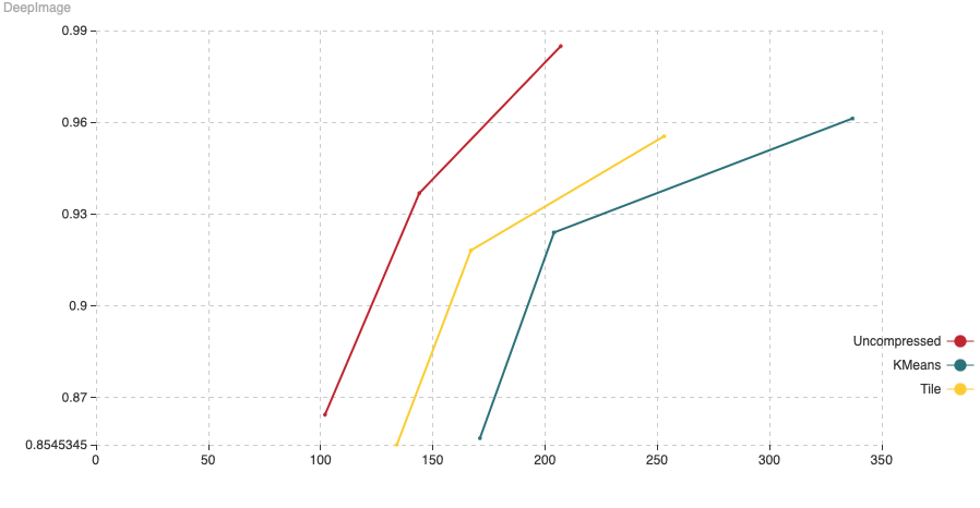 Fig. 7: The chart shows Recall (vertical axis) Vs Indexing time (in minutes, on the horizontal axis). For this experiment we have added 1,000,000 vectors using the normal HNSW algorithm, then we switched to compressed and added the remaining 8,990,000 vectors.
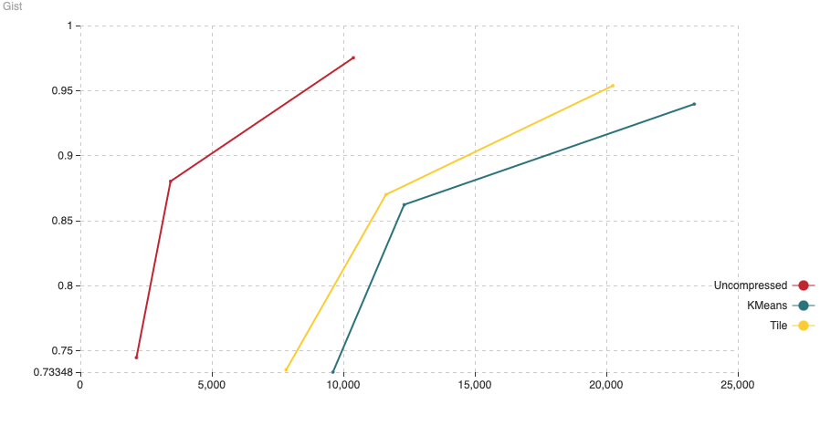 Fig. 8: The chart shows Recall (vertical axis) Vs Latency (in microseconds, on the horizontal axis). For this experiment we have added 200,000 vectors using the normal HNSW algorithm, then we switched to compressed and added the remaining 800,000 vectors.
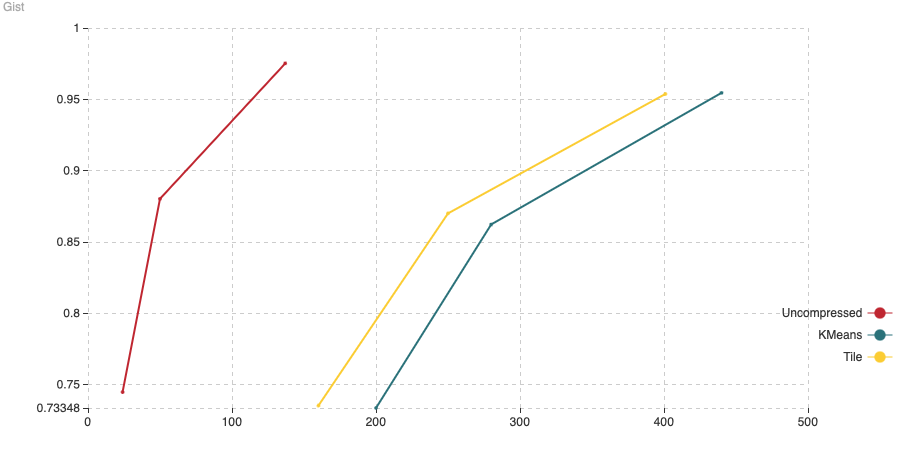 Fig. 9: The chart shows Recall (vertical axis) Vs Indexing time (in minutes, on the horizontal axis). For this experiment we have added 200,000 vectors using the normal HNSW algorithm, then we switched to compressed and added the remaining 800,000 vectors.
Conclusions
In this post we introduced the Tile encoder, an alternative to the KMeans encoder that we mentioned in our last post. Some of the key take away points are that:
- The recall results are very similar when using KMeans vs Tile encoder.
- You need to provide the distribution of your data when using the Tile encoder.
- Fitting with Tile is immediate while it takes much longer with KMeans.
- No downtime when compressing with the Tile encoder, while your server will not be available for querying while compressing with the KMeans encoder.
- You could have the same indexing time when using the Tile encoder if you have enough memory when indexing your data.
Ready to start building?
Check out the Quickstart tutorial, or sign up for a free Weaviate Cloud account.
Don't want to miss another blog post?
Sign up for our bi-weekly newsletter to stay updated!
By submitting, I agree to the Terms of Service and Privacy Policy.