HNSW+PQ - Exploring ANN algorithms Part 2.1

Weaviate is already a very performant and robust vector database and with the recent release of v1.18 we are now bringing vector compression algorithms to Weaviate users everywhere. The main goal of this new feature is to offer similar performance at a fraction of the memory requirements and cost. In this blog we expand on the details behind this delicate balance between recall performance and memory management.

In our previous blog Vamana vs. HNSW - Exploring ANN algorithms Part 1, we explained the challenges and benefits of the Vamana and HNSW indexing algorithms. However, we did not explain the underlying motivation of moving vectors to disk. In this post we explore:

• What kind of information we need to move to disk
• The challenges of moving data to disk
• What the implications of moving information to disk are
• Introduce and test a full first solution offered by the new HNSW+PQ feature in Weaviate v1.18

What Information to Move to disk

When indexing, there exist two big chunks of information that utilize massive amounts of memory: vectors and neighborhood graphs.

Weaviate currently supports vectors of float32. This means we need to allocate 4 bytes, or 32 bits, per stored vector dimension. A database like Sift1M contains 1 million vectors of 128 dimensions each. This means that holding the vectors in memory requires 1,000,000 x 128 x 4 bytes = 512,000,000 bytes.

Additionally, a graph representation of neighborhoods is built when indexing. The graph represents the k-nearest neighbors for each vector. To identify each neighbor we use an int64, meaning we need 8 bytes to store each of the k-nearest neighbors per vector. The parameter controlling the size of the graph is maxConnections. If we use maxConnections = 64 when indexing Sift1M we end up with 1,000,000 x 64 x 8 bytes = 512,000,000 bytes also for the graph. This would bring our total memory requirements to around ~1 GB in order to hold both, the vectors and the graph, for 1,000,000 vectors each with 128 dimensions.

1 GB doesn't sound too bad! Why should we go through the trouble of compressing the vectors at all then!? Sift1M is a rather small dataset. Have a look at some of the other experimental datasets listed in Table 1 below; these are much bigger and this is where the memory requirements can begin to get out of hand. Furthermore, you might be using Weaviate with your own data which might be even bigger than the datasets we report on below. If we extrapolate out, consider how big these memory requirements could grow as you add more objects or represent these objects with long vector embeddings.

DataSet	Dimensions	Vectors	Size in memory (MB)
Sift1M	128	1,000,000	512
Gist	960	1,000,000	3840
DeepImage96	96	9,990,000	3836.16

Table 1: Description of datasets.

Increasing the number of objects vs. storing longer dimensional vectors has an equivalent effect on the overall memory required to store the vectors. As an example consider the Gist dataset, which contains 1,000,000 vectors, each with 960 dimensions. This would mean we need roughly 500 MB for the graph but nearly ten times more memory for the vectors. On the other hand, a database such as DeepImage96 would have 96 dimensions but almost 10,000,000 vectors, meaning, that we would need around 10 GB to hold the vectors and the graph, ~5 GB for each graph.

Our final goal is to move both vectors and graphs to disk. However, we will only explore moving vectors to disk in this post.

Storing vectors on disk is not too challenging. The problem is that moving vectors to disk would have higher latency costs since we would then need lots of disk reads. The proposed solution by DiskANN is to store large complete representations of vectors on disk and keep a compressed representation of them in memory. The compressed representation is used to sort the vectors while searching for the nearest neighbors, and the complete representation is fetched from disk every time we need to explore a new vector from the sorted list.

In plain English, we start our search from our root in the graph. From there, we get a set of neighbor candidates. We need to explore each candidate one at a time. We sort the candidates using the compressed representations, stored in memory, and decide what the best next candidate to explore is. Exploring a candidate would mean fetching it from disk. Notice now that we are not reading all vectors from disk, but only the most promising candidates we wish to explore. This way we still need to host the compressed vectors in memory, but it will give us enough information to reduce disk reads significantly.

The next natural question is: How do we compress vectors?

How to Efficiently Compress Vectors

The main idea behind vector compression is to have a “good-enough” representation of the vectors (as opposed to a perfect representation) so they take up less space in memory while still allowing us to calculate the distance between them in a performant and accurate way. Compression could come from different sources. We could, for example, aim to reduce redundant data to store information more efficiently. We could also sacrifice accuracy in the data in favor of space. We aim to do the latter in this post.

Once we have the data compressed, we still need to be able to calculate distances. This can be accomplished in two ways: Either we compress vectors from the original space to a compressed space to store them and we decompress the vectors back to the original space when calculating the distance, or we define the distance function directly over the compressed space. Figures 1 and 2 graphically demonstrate the first and second options respectively.

Notice the delta($\delta$) term in the explanation. This delta refers to the error we introduce due to the compression - we are using a lossy compression process. As we mentioned before, we are lowering the accuracy of our data, meaning the distance we calculate is a bit distorted; this distortion is exactly what we represent using delta. We don't aim to calculate such an error, nor to try to correct it. We should however acknowledge it and try to keep it low.

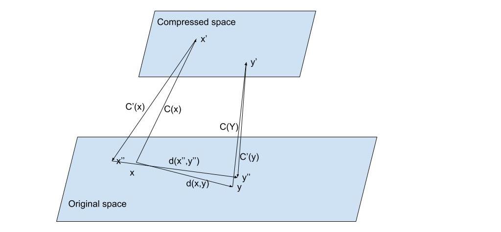Fig. 1: Suppose we have vectors $x$ and $y$ represented in their original space. We apply a compression function $C$ to obtain a shorter representation of $x$ ($x'$) and $y$ ($y'$) on a compressed space but would require a decompression function $C'$ from the compressed space into the original space to be able to use the original distance function. In this case we would obtain $x''$ and $y''$ from $x'$ and $y'$ respectively and apply the distance on the approximations of the original $x$ and $y$ so $d(x,y)=d(x'',y'') + \delta$ where $\delta$ is the distortion added to the distance calculation due of the reconstruction of the original vectors. The compression/decompression mechanisms should be such that the distortion is minimized.

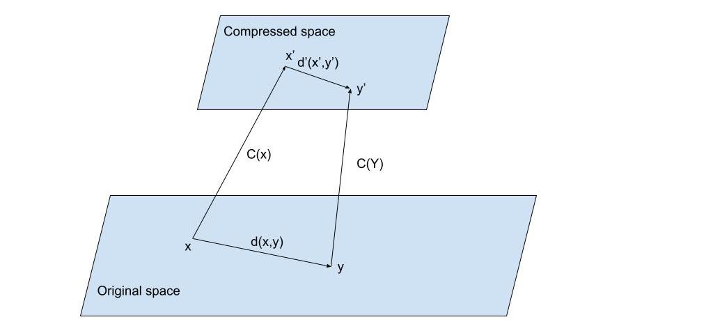Fig. 2: Suppose we have vectors $x$ and $y$ represented in their original space. We apply a compression function $C$ to obtain a shorter representation of $x$ ($x'$) and $y$ ($y'$) on a compressed space. This saves storage space but would require a new distance function $d'$ to operate directly on the compressed space so $d(x,y) = d'(x',y') + \delta$ where $\delta$ is the distortion of the distance. We also need the new distance to be such that the distortion is minimized.

The second approach might be better in terms of performance since it does not require the decompression step. The main problem is that we might need to define a new distance function for each encoding compression function. This solution looks harder to maintain in the long run. The first approach seems more feasible and thus we will explore it next.

In addition to the above mentioned problem, we also need the new functions to operate efficiently so the overall performance of the system doesn't suffer. Keep in mind that for a single query, any ANN algorithm would require distance calculations so by adding unnecessary complexity to the distance function we might severely damage the latency of querying or the overall time to index vectors.

For these reasons we need to select the compression mechanism very carefully! There already exist many compression mechanisms, of which a very popular one is Product Quantization(PQ). This is the compression algorithm we chose to implement in Weaviate with v1.18. Let's explore how PQ works.

Product Quantization

If you already know the details behind how Product Quantization works feel free to skip this section!

The main intuition behind Product Quantization is that it adds the concept of segments to the compression function. Basically, to compress the full vector, we will chop it up and operate on segments of it. For example, if we have a 128 dimensional vector we could chop it up into 32 segments, meaning each segment would contain 4 dimensions. Following this segmentation step we compress each segment independently.

The compression is carried out by using predefined centers, which we will explain shortly. If we aim to compress each segment down to 8 bits (one byte) of memory, we might have 256 (total combinations with 8 bits) predefined centers per segment. When compressing a vector we would go segment-by-segment assigning a byte representing the index of the predefined center. The segmentation and compression process is demonstrated in Figure 3 below.

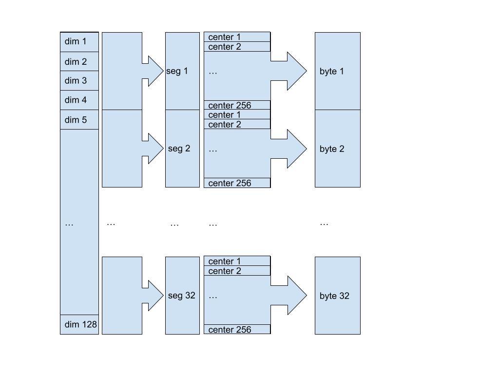Fig. 3: We are compressing a 128 dimensions vector into a 32 bytes compressed vector. For this, we define 32 segments meaning the first segment is composed of the first four dimensions, the second segment goes from dimension 5th to 8th and so on. Then for each segment we need a compression function that takes a four dimensional vector as an input and returns a byte representing the index of the center which best matches the input. The decompression function is straightforward, given a byte, we reconstruct the segment by returning the center at the index encoded by the input.

A straightforward encoding/compression function uses KMeans to generate the centers, each of which can be represented using an id/code and then each incoming vector segment can be assigned the id/code for the center closest to it.

Putting all of this together, the final algorithm would work as follows: Given a set of N vectors, we segment each of them producing smaller dimensional vectors, then apply KMeans clustering per segment over the complete data and find 256 centroids that will be used as predefined centers. When compressing a vector we find the closest centroid per segment and return an array of bytes with the indexes of the centroids per segment. When decompressing a vector, we concatenate the centroids encoded by each byte on the array.

The explanation above is a simplification of the complete algorithm, as we also need to be concerned about performance for which we need to address duplication of calculations, synchronization in multithreading and so on. However what we have covered above should be sufficient to understand what you can accomplish using the PQ feature released in v1.18. Let's see some of the results HNSW implemented with PQ in Weaviate can accomplish next! If you're interested in learning more about PQ you can refer to the documentation here. If you want to learn how to configure Weaviate to use PQ refer to the docs here.

KMeans encoding results

First, the PQ feature added to version 1.18 of Weaviate is assessed in the sections below. To check performance and distortion, we compared our implementation to NanoPQ and we observed similar results.

The main idea behind running these experiments is to explore how PQ compression would affect our current indexing algorithms. The experiments consist of fitting the Product Quantizer on some datasets and then calculating the recall by applying brute force search on the compressed vectors. This will give us two important results, the time it would take to fit the data with KMeans clustering and compress the vectors (which will be needed at some step by the indexing algorithm) and the distortion introduced by reconstructing the compressed vectors to calculate the distance. This distortion is measured in terms of a drop in recall.

We considered three datasets for this study: Sift1M, Gist1M and DeepImage 96. Table 1, shown above, summarizes these datasets. To avoid overfitting, and because this is how we intend to use it in combination with the indexing algorithm, we use only 200,000 vectors to fit KMeans and the complete data to calculate the recall.

We analyze Product Quantization with KMeans encoding using different segment lengths. Notice that the lengths for the segments should be an integer divisor of the total amount of dimensions. For Sift1M we have used 1, 2, 4 and 8 dimensions per segment, while for Gist and DeepImage we have used 1, 2, 3, 4 and 6 dimensions per segment. Using segment length of 1 on Sift1M would give us 128 segments, while a segment length of 8 would give us 16 segments.

We also offer the flexibility of choosing the amount of centroids to use with KMeans. The compression rate will depend on the amount of centroids. If we use 256 centroids we only need one byte per segment. Additionally, using an amount in the range 257 to 65536 will require two bytes per segment.

Sift

First, we show results on Sift1M. We vary the amount of centroids starting with 256 and increase the number until it performs poorly compared to the next curve. Notice that similar recall/latency results with less segments still mean better compression rate.

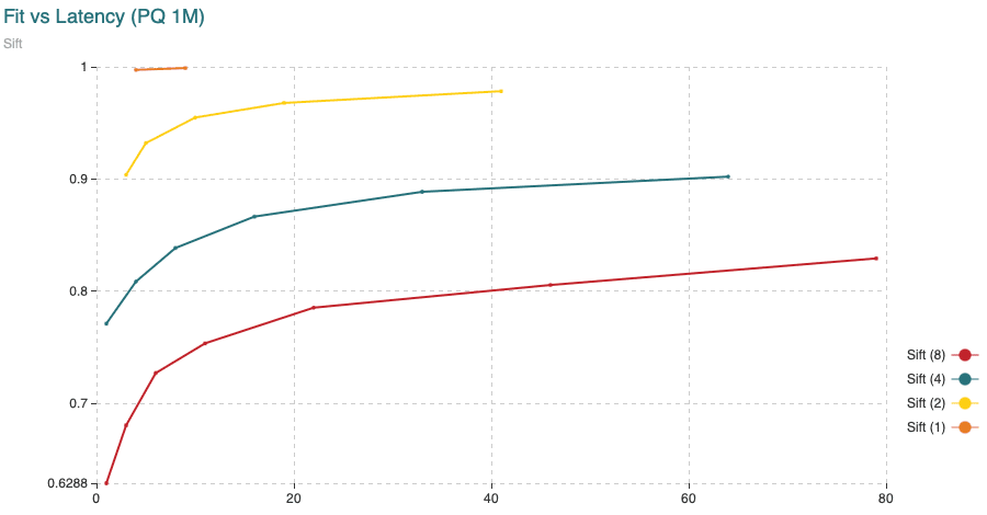Fig. 4: Time (min) to fit the Product Quantizer with 200,000 vectors and to encode 1,000,000 vectors, all compared to the recall achieved. The different curves are obtained varying the segment length (shown in the legend) from 1 to 8 dimensions per segment. The points in the curve are obtained varying the amount of centroids.

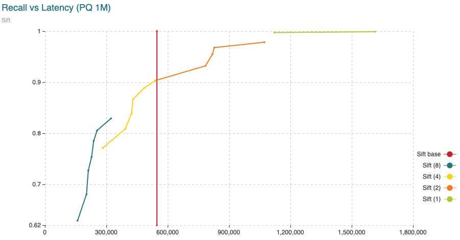Fig. 5: Average time (microseconds) to calculate distances from query vectors to all 1,000,000 vectors compared to the recall achieved. The different curves are obtained varying the segment length (shown in the legend) from 1 to 8 dimensions per segment. The points in the curve are obtained varying the amount of centroids. The “base” curve refers to the fixed average time to calculate distances between uncompressed vectors.

Notice some important findings from the experiments. Latency could vary significantly depending on the settings we use. We could reduce latency by paying some penalty in the distortion of the distances (observed in the recall drop) or we could aim for more accurate results with a higher latency penalty.

Deep-Image

Next we show the results on DeepImage96. We see a similar profile compared to Sift1M. Latency is nearly 10 times slower but this is due to the fact that we have nearly 10 times more vectors.

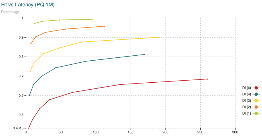Fig. 6: Time (min) to fit the Product Quantizer with 200,000 vectors and to encode 9,990,000 vectors, all compared to the recall achieved. The different curves are obtained varying the segment length (shown in the legend) from 1 to 6 dimensions per segment. The points in the curve are obtained varying the amount of centroids.

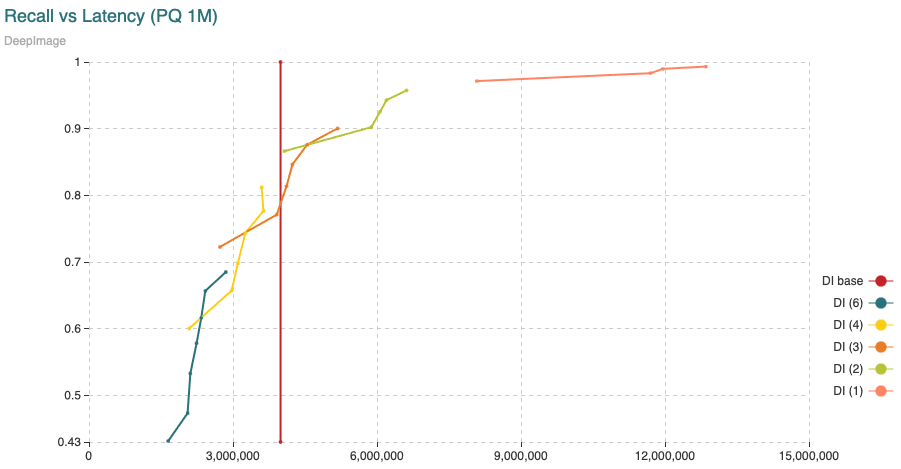Fig. 7: Average time (microseconds) to calculate distances from query vectors to all 9,990,000 vectors compared to the recall achieved. The different curves are obtained varying the segment length (shown in the legend) from 1 to 6 dimensions per segment. The points in the curve are obtained varying the amount of centroids. The “base” curve refers to the fixed average time to calculate distances between uncompressed vectors.

Gist

Finally, we show results on the Gist database using the 1,000,000 vectors. We see a similar profile compared to Sift1M again. Latency is nearly 10 times slower but this time it is due to the fact that we have nearly 10 times more dimensions per vectors.

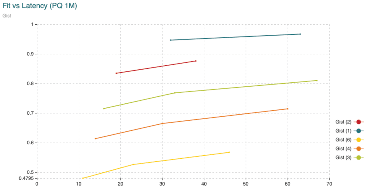Fig. 8: Time (min) to fit the Product Quantizer with 200,000 vectors and to encode 1,000,000 vectors, all compared to the recall achieved. The different curves are obtained varying the segment length (shown in the legend) from 1 to 6 dimensions per segment. The points in the curve are obtained varying the amount of centroids.

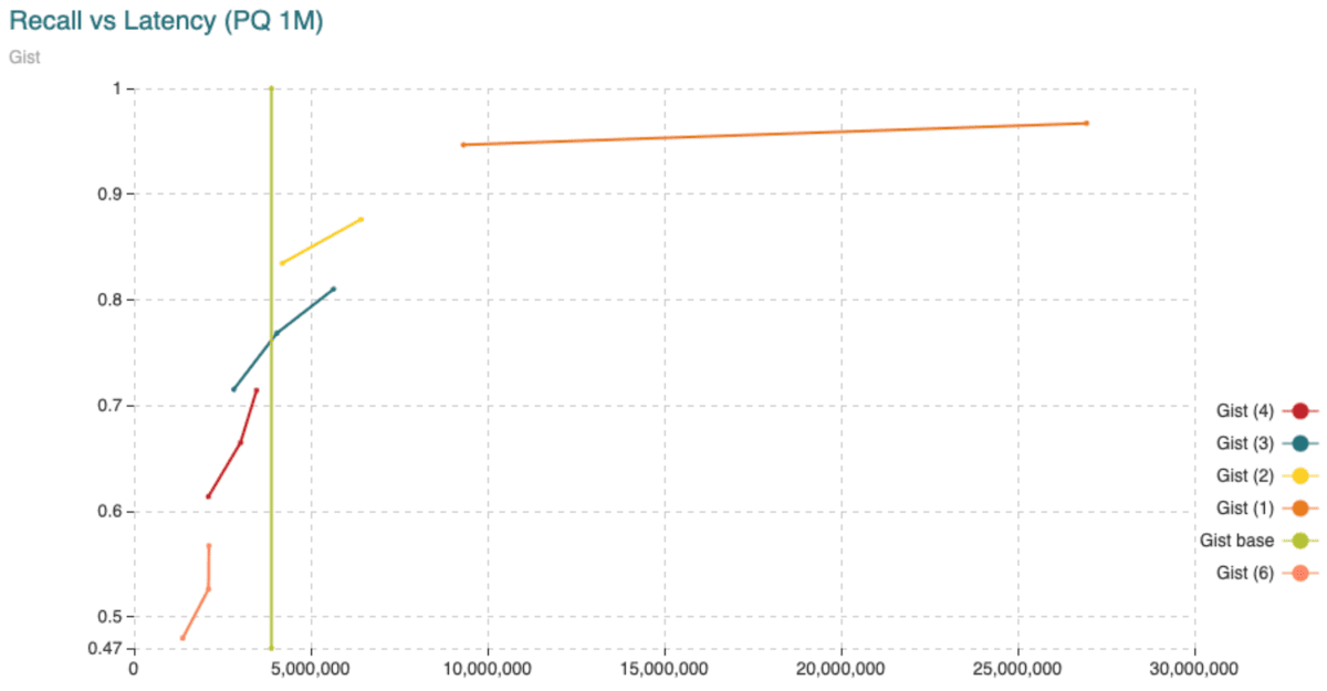Fig. 9: Average time (microseconds) to calculate distances from query vectors to all 1,000,000 vectors compared to the recall achieved. The different curves are obtained varying the segment length (shown in the legend) from 1 to 6 dimensions per segment. The points in the curve are obtained varying the amount of centroids. The “base” curve refers to the fixed average time to calculate distances between uncompressed vectors.

As we should expect, Product Quantization is very useful for saving memory. It comes at a cost though. The most expensive part is fitting the KMeans clustering algorithm. To remedy this we could use a different encoder based on the distribution of the data, however that is a topic we shall save for later!

A final word on performance, not all applications require a high recall. Sometimes, it's enough to output relevant data really fast. In such cases we care about latency a lot more than recall. Compressing, not only saves memory but also time. As an example, consider brute force where we compress very aggressively. This would mean we do not need memory at all for indexing data and very little memory for holding the vectors. The main metric of concern in this setting is the latency with which we can obtain our replies. Product Quantization not only helps with reducing memory requirements in this case but also with cutting down on latency. The following table compares improvement in latency that can be achieved using PQ aggressively.

Dataset	Segments	Centroids	Compression		Latency (ms)
Sift	8	256	x64	Compressed	46 (x12)
				Uncompressed	547
DeepImage	8	256	x48	Compressed	468 (x8.5)
				Uncompressed	3990
Gist	48	256	x80	Compressed	221 (x17.5)
				Uncompressed	3889

Tab. 2: Brute force search latency with high compression ratio.

HNSW+PQ

Our complete implementation of FreshDiskANN still requires a few key pieces, however at this point we have released the HNSW+PQ implementation with v1.18 for our users to take advantage of. This feature allows HNSW to work directly with compressed vectors. This means using Product Quantization to compress vectors and calculate distances.

As mentioned before, we could still store the complete representation of the vectors on disk and use them to correct the distances as we explore nodes during querying. For the time being, we are implementing only HNSW+PQ which means we do no correction to the distances. In the future we will explore adding such a correction and see the implications in recall and latency since we will have more accurate distances but also much more disk reads.

We could use regular HNSW to start building our index. Once we have added some vectors (a fifth of the total amount, for example) we could then compress the existing vectors and from this point on, we compress the vectors once they come into the index. The separation between loading data uncompressed, then compressing afterwards is necessary. The threshold of how much data needs to be loaded in prior to compressing (a fifth of the data) is not a rule though. The decision on when to compress should be taken keeping in mind that we need to send enough data for the Product Quantizer to infer the distribution of the data before actually compressing the vectors. If we compress too soon, when too little data is present in uncompressed form, the centroids will be underfit and won't capture the underlying data distribution. Alternatively, compressing too late will take up unnecessary ammounts of memory prior to compression. Keep in mind that the uncompressed vectors will require more memory so if we send the entire dataset and compress only at the end we will need to host all of these vectors in memory at some point prior to compressing after which we can free that memory. Depending on the size of your vectors the compressing time could be optimally calculated but this is not a big issue either.

Figure 10 shows a profile of the memory used while loading Sift1M. Notice the first peak in memory at the beginning. This was the memory used for loading the first fifth of the data plus compressing the data. We then wait for the garbage collection cycle to claim the memory back after which we send the remaining data to the server. Note that the peaks in the middle are due to memory not being freed by the garbage collection process immediately. At the end you see the actual memory used after the garbage collection process clean everything up.

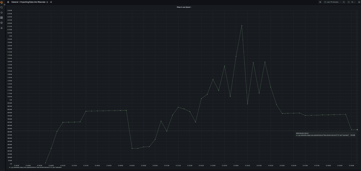Fig. 10: Heap usage while loading the data into the Weaviate server. Memory does not grow smoothly. Instead there is a higher peak at the beginning before the vectors are compressed.

Lets focus the comparison in three directions:

• How much longer does it take to index compressed data?
• How much does it affect the recall and latency?
• How much do we save in memory requirements?

Performance Results

In the following figures we show the performance of HNSW+PQ on the three databases used above. Notice how compressing with KMeans keeps the recall closer to the uncompressed results. Compressing too aggressively (KMeans with a few dimensions per segment) improves memory, indexing and latency performance but it rapidly destroys the recall so we recommend using it discreetly. Notice also that KMeans encoding with as many segments as dimensions ensures a 4 to 1 compression ratio. The next segment amounts ensure 8, 16 and 32 to 1 compression ratio (in the case of sift which uses 2, 4 and 8 dimensions per segment).

All experiments were performed adding 200,000 vectors using uncompressed behavior, then compressing and adding the rest of the data.

We do not include the same charts for DeepImage but results are similar to those obtained over Sift1M.

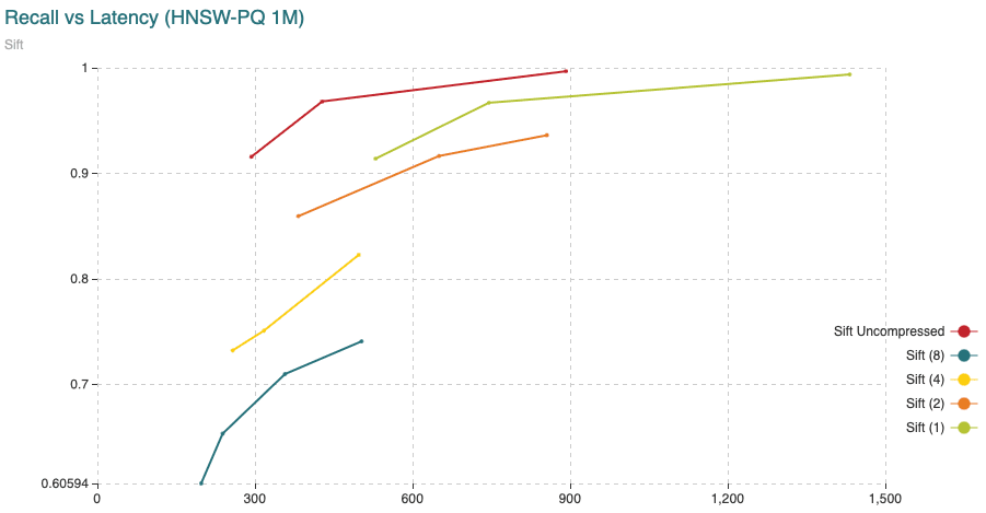Fig. 11: The chart shows Recall (vertical axis) Vs Latency (in microseconds, on the horizontal axis). For this experiment we have added 200,000 vectors using the normal HNSW algorithm, then we switched to compressed and added the remaining 800,000 vectors.

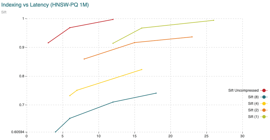Fig. 12: The chart shows Recall (vertical axis) Vs Indexing time (in minutes, on the horizontal axis). For this experiment we have added 200,000 vectors using the normal HNSW algorithm, then we switched to compressed and added the remaining 800,000 vectors.

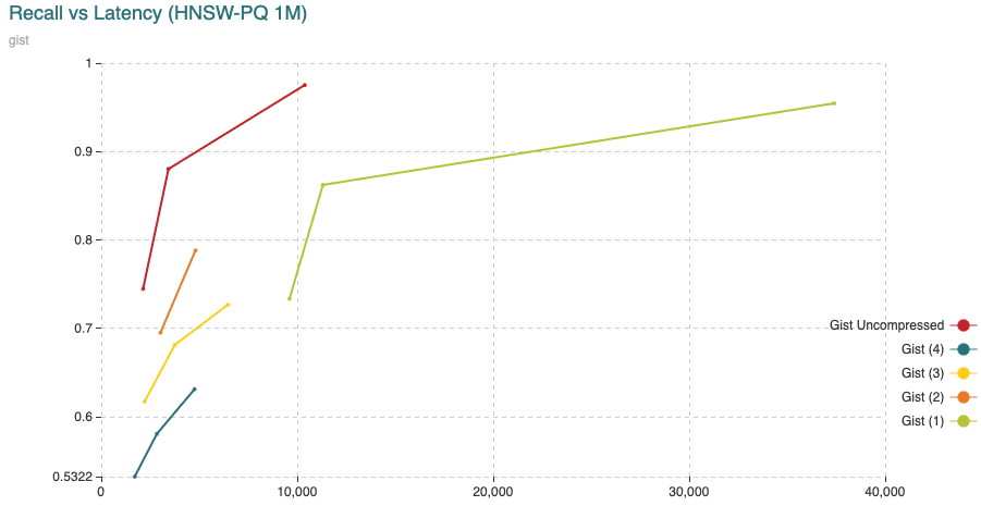Fig. 13: The chart shows Recall (vertical axis) Vs Latency (in microseconds, on the horizontal axis). For this experiment we have added 200,000 vectors using the normal HNSW algorithm, then we switched to compressed and added the remaining 800,000 vectors.

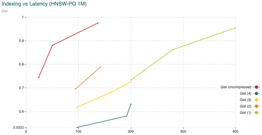Fig. 14: The chart shows Recall (vertical axis) Vs Indexing time (in minutes, on the horizontal axis). For this experiment we have added 200,000 vectors using the normal HNSW algorithm, then we switched to compressed and added the remaining 800,000 vectors.

Memory compression results

To explore how the memory usage changes with the HNSW+PQ feature, we compare the two versions: uncompressed HNSW and HNSW plus compression using the KMeans encoder. We only compare KMeans using the same amount of segments as dimensions. All other settings could achieve a little bit of a higher compression rate but since we do not compress the graph, it is not significant for these datasets. Keep in mind that the whole graph built by HNSW is still hosted in memory. As we have mentioned before, this is not the final solution where we still do not move information to disk. Our final solution would use a compressed version of the vectors to guide the exploration and fetch the fully described data (vectors and graph) from disk as needed. With the final approach we will achieve better compression rate but also better recall since the uncompressed vectors will be used to correct the compression distortion. A final remark. Notice how the compression rate is better on Gist. The reason for this is the fact that we have larger vectors. This means that the memory dedicated to vectors is larger than the memory dedicated to the graph and since we only compress vectors, then the larger the vectors the higher the compression rate. Having even larger vectors such as OpenAI embeddings (1536 dimensions) would reach even better compression rates.

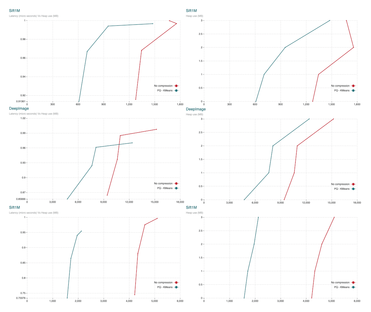Fig.15: The charts show heap usage. Top down it shows Sift1M, DeepImage and Gist. Charts to the left show Recall (vertical axis) Vs Heap usage (horizontal axis). Charts to the right show Heap usage (horizontal axis) Vs the different parameter sets. Parameter sets to achieve a larger graph (also producing a more accurate search) are charted from top down.

Let's sumamrize what we see in the above charts. We could index our data using high or low parameters set. Additionally, we could aim for different levels of compression. The fact that the graph is still in memory makes it hard to see the difference between those different levels of compression. The more we compress the lower the recall we would expect. Let us discuss the lowest level of compression along with some expectations.

For Sift1M we would require roughly 1277 MB to 1674 MB of memory to index our data using uncompressed HNSW. This version would give us recall ranging from 0.96811 to 0.99974 and latencies ranging from 293 to 1772 microseconds. If we compress the vectors then the memory requirements goes down to 610 MB to 1478 MB range. After compression recall, drops to values ranging from 0.9136 to 0.9965. Latency rises up to the 401 to 1937 microsends range.

For DeepImage96 we would require roughly 9420 MB to 15226 MB of memory to index our data using uncompressed HNSW. This version would give us recall ranging from 0.8644 to 0.99757 and latencies ranging from 827 to 2601 microseconds. If we compress the vectors then the memory requirements goes down to the 4730 MB to 12367 MB range. After compression, recall drops to values ranging from 0.8566 to 0.9702. Latency rises up to the 1039 to 2708 microsends range.

For Gist we would require roughly 4218 MB to 5103 MB of memory to index our data using uncompressed HNSW. This version would give us recall ranging from 0.7446 to 0.9962 and latencies ranging from 2133 to 15539 microseconds. If we compress the vectors then the memory requirements goes down to the 1572 MB to 2129 MB range. After compression, recall drops to values ranging from 0.7337 to 0.9545. Latency rises up to the 7521 to 37402 microsends range.

A summary is shown in Table 3 below.

		Recall100@100	Latency ($\mu s$)	Memory required (MB)
Sift1M Low params	Uncompressed	0.91561	293	1277
	Compressed	0.91361	401 (x1.36)	610 (47.76%)
Sift1M High params	Uncompressed	0.99974	1772	1674
	Compressed	0.99658	1937 (x1.09)	1478 (88.29%)
DeepImage Low params	Uncompressed	0.8644	827	9420
	Compressed	0.85666	1039 (x1.25)	4730 (50.21%)
DeepImage High params	Uncompressed	0.99757	2601	15226
	Compressed	0.97023	2708 (x1.04)	12367 (81.22%)
Gist Low params	Uncompressed	0.74461	2133	4218
	Compressed	0.73376	7521 (x3.52)	1572 (37.26%)
Gist High params	Uncompressed	0.99628	15539	5103
	Compressed	0.95455	37402 (x2.40)	2129 (41.72%)

Tab. 3: Summary of the previously presented results. We show results for the shortest and largest parameter sets for uncompressed and compressed versions. Additionally we show the speed down rate in latency and the percentage of memory, compared to uncompressed, needed to operate under compressed options.

We would like to give you an extra bonus row from the above table. Sphere is an open-source dataset recently released by Meta. It collects 768 dimensions and nearly a billion objects. Only hosting the vectors in memory would take 3.1 TB. To work with data of this size, either you need to spend more to provision expensive resources, or you can sacrifice a bit on recall and latency and save drastically on resources.

We show a simple test below to drive home the importance of compressing data and eventually moving graphs also to disk. The test was run over 10 million objects only. A final note on the numbers. While all the experiments above have been carried out directly on the algorithm, the table below is constructed using data collected from interactions with the Weaviate server. This means the latency is calculated end to end (with all the overhead on communication from clients).

		Latency (ms)	Memory required (GB)	Memory to host the vectors (GB)
10M vectors from Sphere	Uncompressed	119	32.54	28.66
	Compressed (4-to-1)	273 (x2.29)	10.57 (32.48%)	7.16 (24.98%)

Tab. 4: Summary of latency and memory requirements on the 10M Sphere subset. Additionally we show the speed down rate in latency and the percentage of memory, compared to uncompressed, needed to operate under compressed options.

Conclusions

In this post we explore the journey and details behind the HNSW+PQ feature released in Weaviate v1.18. Though we still have a ways to go on this journey, as noted earlier, but what we've accomplished thus far can add loads of value to Weaviate users. This solution already allows for significant savings in terms of memory. When compressing vectors ranging from 100 to 1000 dimensions you can save half to three fourths of the memory you would normally need to run HNSW. This saving comes with a little cost in recall or latency. The indexing time is also larger but to address this we've cooked up a second encoder, developed specially by Weaviate, based on the distribution of the data that will reduce the indexing time significantly. Keep your eyes peeled for more details on this soon on our blog! We will share our insights as we go. 😀

Ready to start building?

Check out the Quickstart tutorial, or build amazing apps with a free trial of Weaviate Cloud (WCD).

GitHub

Forum

Slack

X (Twitter)

Don't want to miss another blog post?

Sign up for our bi-weekly newsletter to stay updated!

By submitting, I agree to the Terms of Service and Privacy Policy.