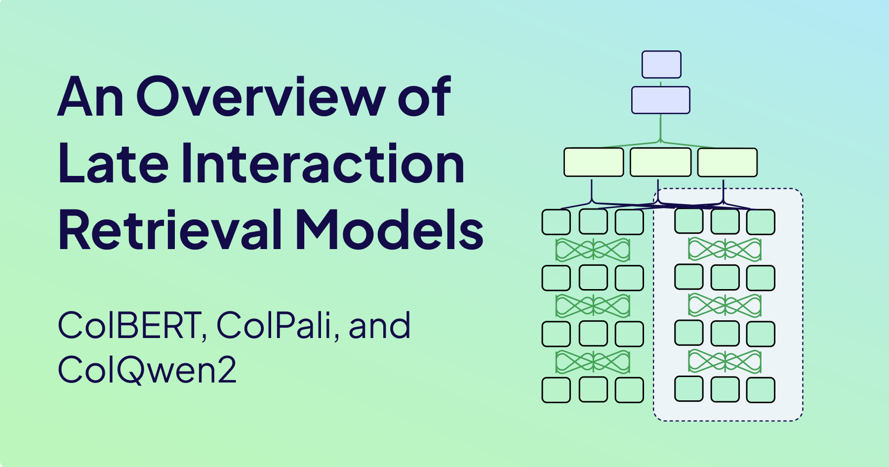
An Overview of Late Interaction Retrieval Models: ColBERT, ColPali, and ColQwen

Why Late Interaction?

Late interaction retrieval models are changing how we find and retrieve information. These models allow for semantically rich interactions that enable a precise retrieval process across different modalities of unstructured data, including text and images. By decomposing query and document embeddings into lower-level representations, late interaction models use multi-vector retrieval and improve both accuracy and scalability compared to no-interaction and full-interaction dense retrieval models.

Late interaction models can be used across various retrieval tasks, helping researchers and practitioners find relevant documents in large document collections, such as financial documents or legal contracts. These models are particularly helpful in downstream tasks requiring efficient retrieval processes, such as search engines or Generative AI applications, such as Retrieval-Augmented Generation (RAG) pipelines, where semantic precision can improve information extraction and understanding.

3 Types of Interaction in Dense Retrieval Models

Dense retrieval models can be categorized based on their type of “interaction”. A dense retrieval model is a model that uses some type of neural network architecture to retrieve relevant documents for a search query. In this context, “interaction” refers to the process of assessing how well a document matches a given search query by comparing their representations. This section discusses the different types of interactions in dense retrieval models.

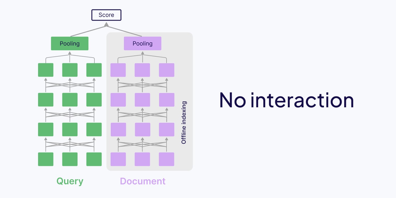
No-interaction Retrieval Models

Traditional methods for retrieval commonly use “no-interaction” retrieval models. In this case, the search query and documents are processed separately:

1. During the indexing phase, one dense vector embedding is precomputed for each document. The document is first split up into separate tokens, all tokens are passed together through a neural network model, typically a transformer model, to obtain separate dense embeddings for each token. Finally, the token embeddings are calculated into a single vector representation via pooling.
2. During the online querying phase, one vector is computed for the search query to search for similar documents from the pre-computed document embeddings with a similarity metric (e.g., dot product, cosine similarity).

Advantages of no-interaction retrieval models are primarily that they are fast and computationally efficient. The vector representations of the documents are already pre-computed and indexed offline, and at query time, only the query embeddings have to be computed. This makes this solution scalable for large-scale information retrieval systems and vector search applications.

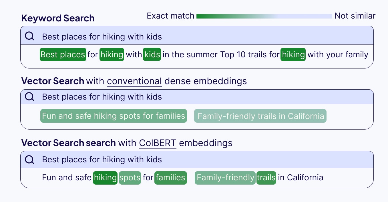
Disadvantages of no-interaction retrieval models lie in the lack of interaction between the search query and the documents. Because the search query and the documents are processed separately and compressed into single vector embeddings, this approach can miss contextual nuances. Any contextual nuances shared from one token to another have to be compressed before the comparison takes place - meaning similarity is compared between the whole document and the whole query, rather than on a token-by-token level.

These characteristics make no-interaction models great for first-stage retrieval, where candidates are retrieved from a large document collection, like in vector search. Examples of no-interaction retrieval models are bi-encoders, such as OpenAI’s text-embedding-3-small.

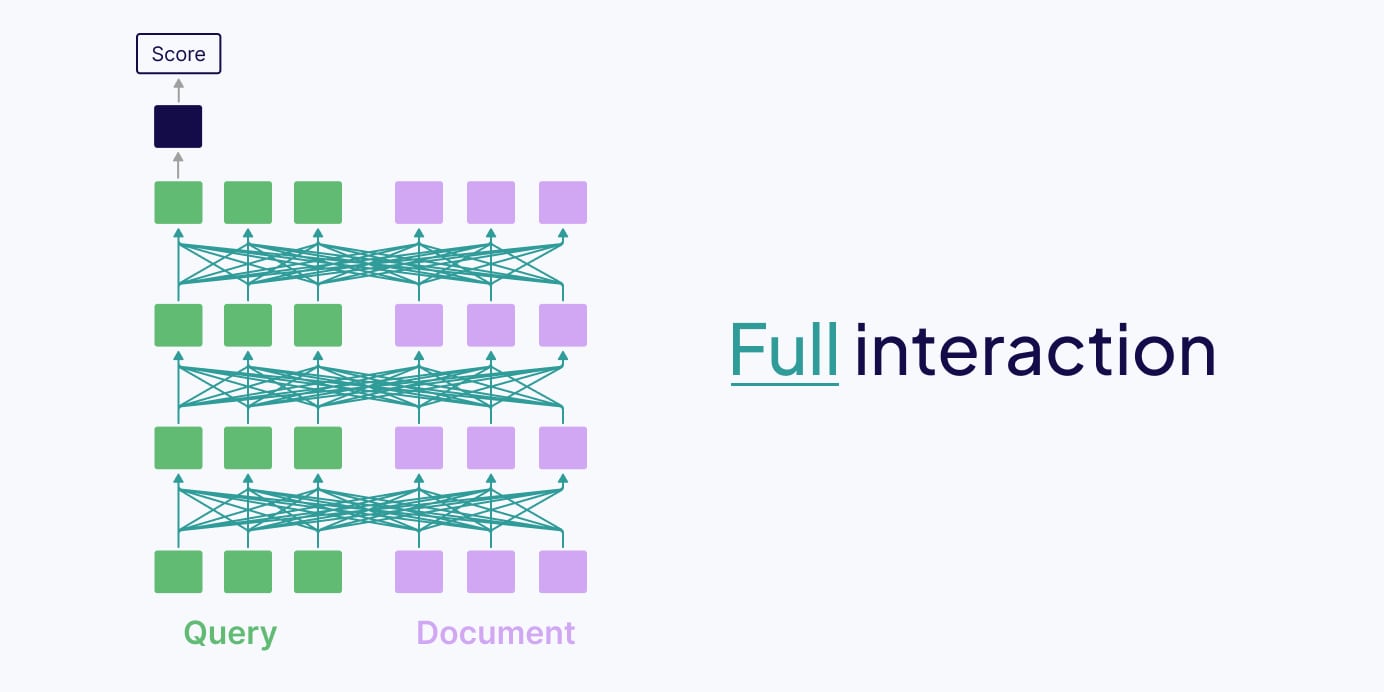
Full interaction Retrieval Models

Full interaction retrieval models process the search query and documents together. That’s why they are sometimes also called early interaction or all-to-all interaction retrieval models. In contrast to no-interaction models, all-to-all interaction models process everything at query time. For this, the query is concatenated with each document, and then they are processed together for full cross-attention.

Advantages of full interaction retrieval models stem from them being contextually rich, meaning they effectively capture nuanced contextual relationships between the search query and the document.

Disadvantages of full interaction models are due to them being extremely computationally expensive because all documents have to be processed at query time. That’s why full interaction models are not scalable for large amounts of documents.

These characteristics make full interaction models great for second-stage retrieval, like reranking a curated set of candidate documents. Examples of full interaction retrieval models are BERT and other models with cross-encoder architectures, which are often popular in reranking models.

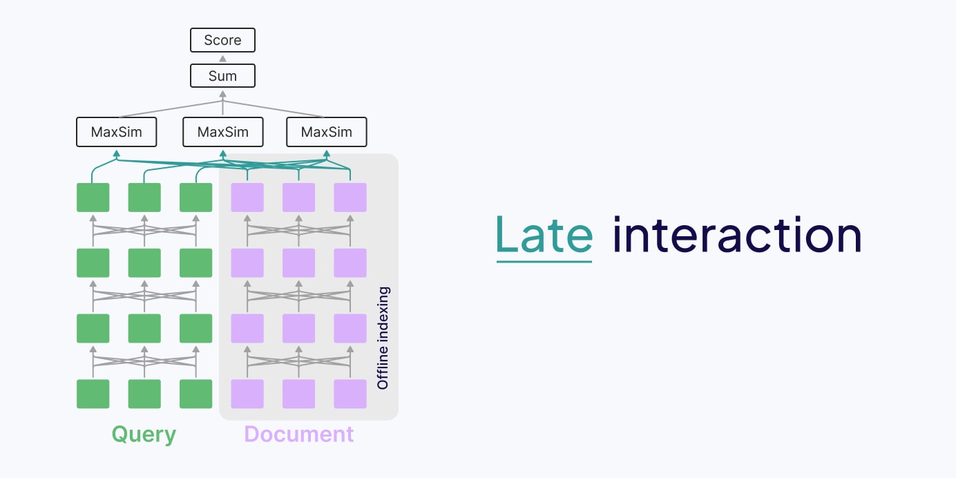
Late interaction retrieval models

Whilst no-interaction models are fast but can be inaccurate, all-to-all interaction models are accurate but slow, late interaction retrieval models promise to be both. Late interaction models are inspired by both of the above retrieval models.

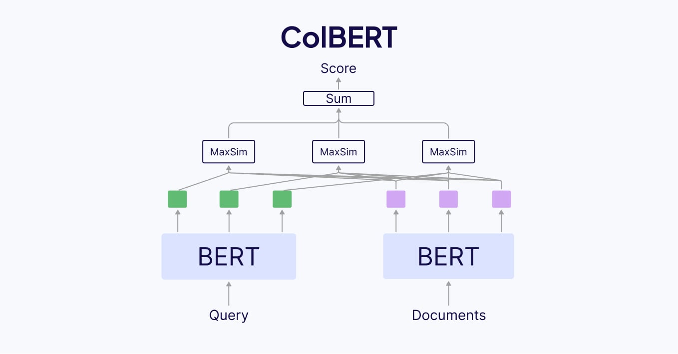
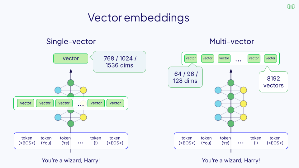
Similar to no-interaction retrieval models, late interaction models have a dual encoder architecture and precompute embeddings for each document offline (in advance of the interaction stage). However, in late interaction, the embeddings that are stored are for each token, rather than a single embedding for the whole document. Instead of pooling these token embeddings, the pooling mechanism is replaced with the late interaction mechanism. That means that the token-level multi-vector embeddings are kept to calculate the interaction between the search query and document multi-vector representations, similar to full interaction retrieval models, but at a later stage.

Advantages of late interaction retrieval models are that they are both scalable and contextually rich.

Disadvantages of late interaction are related to their storage requirements - they require an embedding for each token, which requires a lot more storage for a complete set of vectors.

However, token embeddings can be stored at a much lower dimension and quantization level to decrease computational costs and increase storage efficiency - mitigating some of these issues. For example, in ColBERTv2, aggressive quantization is performed to reduce the size of each vector from 256 bytes to 36 bytes (2-bit compression) or even 20 bytes (1-bit compression), whilst maintaining a good level of accuracy (see the ColBERTv2 section later).

Examples of late interaction retrieval models are ColBERT, ColPali, and ColQwen, which are discussed in the following sections.

How does the late interaction mechanism work?

The late interaction mechanism calculates the maximum similarity score between the query tokens and the document tokens. It requires lower-level representations of input documents or images, such as their tokens (word parts) or image patches (small image/document sections), and uses these for comparison instead of a global document representation. Late interaction was first introduced in the ColBERT paper.

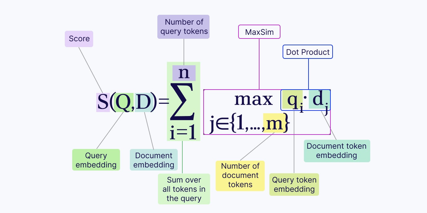
Let’s say we have a text query and text documents, for simplicity of explanation. Instead of pooling the vector embeddings into a single vector representation for the query and the document, we keep the token-level embeddings and apply the MaxSim operator to calculate the relevance scores:

1. For each query token, we compute its similarity score (e.g., dot product or cosine similarity) with every document token.
2. Then, for each query token, we keep only the maximum similarity score (e.g., maximum dot product or maximum cosine similarity).
3. Finally, we sum all of those token-level maximum similarity scores into a final relevance score.

What is ColBERT?

The ColBERT paper, released in 2020, introduced both the original ColBERT model and the late interaction mechanism. ColBERT stands for “Contextualized Late Interaction over BERT”. It is a model fine-tuned on the BERT language model, which was one of the first big transformer models in NLP. ColBERT however uses the late interaction mechanism instead of the typical all-to-all interaction that BERT uses, and is specialized towards generating contextualized embeddings for queries and documents. Since BERT is a text-only model (not multimodal), ColBERT is also a text-only model.

Fun fact: It’s pronounced /koʊlˈbɛər after Stephen Colbert in reference to his Late Show.

ColBERT Model Architecture

Since ColBERT is a fine-tune of BERT, its architecture is almost identical to BERT. BERT-base was trained with 110M parameters (340M for BERT-large), and different variations of ColBERT were trained from BERT-base and BERT-large on different training datasets. The version of ColBERT you’ll find on Hugging Face is fine-tuned from BERT-base and has around 110M parameters.

However, there are a few differences between ColBERT and BERT. Firstly, BERT-base used a fixed embedding dimension of 768 (1024 for BERT-large), whereas ColBERT uses a smaller representation dimension of 128 for each vector in an effort to reduce the storage requirements of each vector. This is achieved via a projection layer in ColBERT to make the final output a 128-dimensional vector.

The same fine-tuned BERT model is used in ColBERT as both the query encoder and the document encoder separately, but two additional special tokens, [Q] and [D], are prepended to the query and document respectively to 'mark' them as such. This marker is included in model training, so that the model learns to distinguish the query and document via these special tokens.

A full forward pass of ColBERT is given in order by:

1. Tokenize the query/document (and include special token [Q] or [D])
2. Pass the tokens through a 110M fine-tuned BERT-base transformer model
3. Project the final BERT representations with a special projection layer to reduce the embedding dimension to 128 instead of 768
4. Compare all tokens between query and document using late interaction and MaxSim.

ColBERT v2 and its improvements

Whilst ColBERT introduced the concept of late interaction, ColBERTv2 refined it. The main downside of ColBERT is the storage requirements - needing a full vector for each token in each document. ColBERTv2 improves over the original ColBERT’s weakness of huge memory storage requirements, whilst also improving the quality of retrieval.

The increased quality of ColBERTv2 comes from a process called denoised supervision, which involves distillation (passing on knowledge) from a larger teacher model and hard negative mining (showing similar but incorrect retrievals to a given query).

Distillation was from the teacher model, MiniLM. This cross-encoder model uses all-to-all interaction, like BERT, which means it has a high accuracy but is more inefficient to use in practice. Distillation means that this model can be used to teach ColBERTv2, whilst ColBERTv2 retains its increased computational efficiency thanks to late interaction.

Hard negative mining involves framing the retrieval with documents that are similar, but not relevant to, the query, so the model learns to distinguish between the correct document, and documents similar to this correct one. This reduces the number of false negatives ColBERTv2 will retrieve.

The improved storage efficiency of ColBERTv2 comes from residual compression. Residual compression is a technique which stores ‘centroids’ in high precision (more accurate vectors with high storage cost), and ‘residual’ vectors in low precision (less accurate vectors with lower storage cost). Each token embedding is a combination of a centroid and its own, unique, residual vector. These vector centroids take up more space but there are fewer of them; according to the ColBERTv2 paper, they recommend using

$$\lfloor16 \times \sqrt{n_{docs} \times d_{embedding}}\rfloor$$

many vectors, which is a value proportional to the number of overall embeddings in the dataset.

Using this residual compression technique reduces the space footprint massively - the MS MARCO training dataset had a 154GB index on ColBERTv1, whereas on COLBERTv2 this technique allowed it to be stored as low as 16GB for 1-bit compression, or 25GB for 2-bit compression. The space footprint from ColBERTv2 was reduced by 6-10x compared to ColBERTv1, and brings this value closer to what a typical single vector model would require for this dataset.

Advantages and Limitations of ColBERT

One advantage of ColBERT is its impact on retrieval performance. Because it’s scalable and contextually rich, it can improve retrieval accuracy and, therefore, overall performance in RAG applications and ranking pipelines compared to typical dense vector embedding models.

Another positive side-effect of keeping token-level embeddings for similarity scoring in ColBERT is an added feature of explainability. Similar to keyword matching, you can get more interpretable insights for your vector search results because you can see which tokens have a high similarity score between the search query and the relevant document.

However, the multi-vector approach of the original ColBERT model has one big disadvantage of the increased space footprint. Because with ColBERT you now have one vector embedding for each token in a document instead of one vector embedding for one document, the storage requirements and memory usage balloon up, but this can be mitigated somewhat with the quantization methods introduced by ColBERTv2.

Let’s compare the storage requirements of dense vector embeddings and multi-vector embeddings. Assume that each document consists of 100 tokens, and we are storing a variable number of documents. The table below gives the storage cost, in megabytes, to store all of the documents as their respective embeddings.

The storage costs calculated assume that each value in the single vector embedding is quantized slightly at 16-bits per dimension, and the multi-vector embedding is heavily quantized to 2-bits per dimension, with the centroids assumed as 16-bit precision, and the number of centroids is given by the formula in the previous section.

		Single Vector Embeddings			Multi Vector Embeddings (ColBERTv2 quantization)
		d=768	d=1024	d=1536	d=64	d=96	d=128
Number of Documents (n) (100 tokens per document)	n=100	0.15 MB	0.20 MB	0.31 MB	0.36 MB	0.55 MB	0.73 MB
	n=500	0.77 MB	1.02 MB	1.54 MB	1.26 MB	1.89 MB	2.52 MB
	n=1000	1.54 MB	2.05 MB	3.07 MB	2.25 MB	3.37 MB	4.50 MB
	n=2000	3.07 MB	4.10 MB	6.14 MB	4.12 MB	6.17 MB	8.23 MB
	n=10000	15.36 MB	20.48 MB	30.72 MB	18.05 MB	27.07 MB	36.10 MB

Even with heavy quantization, storing 128-dimensional vectors with ColBERTv2 costs significantly more than storing a high-dimensional single vector for the entire document/chunk. As the size of the documents and the number of tokens scale up, the storage cost will also balloon, which could be unsustainable for some scenarios. However, the increased contextual richness and retrieval performance may well be worth the extra storage.

Use Cases of ColBERT

Because of its improved correlation of textual nuances, ColBERT is great for retrieval tasks that require a higher level of accuracy, like legal text-based RAG pipelines or financial document verification.

You can find a RAG code example with ColBERT in Python in our documentation.

What are ColPali and ColQwen?

ColPali and ColQwen are multimodal late interaction retrieval models that use vision language models (VLMs) instead of text-only models. ColPali stands for Contextualized Late Interaction over PaliGemma, while ColQwen stands for Contextualized Late Interaction over Qwen2 (that’s why it’s also called ColQwen2).

Unlike conventional approaches to PDF retrieval that require Optical Character Recognition (OCR) and advanced chunking to separate different content formats (i.e textual content and visual content, like graphs or images) when doing complex document processing, ColPali and ColQwen treat the entire PDF as an image, and thus these models extend ColBERT's concept to visual content.

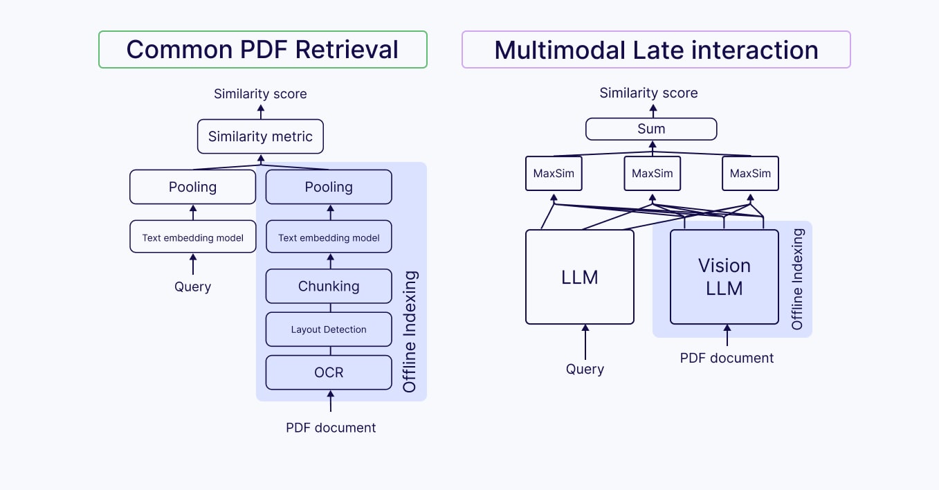
ColPali and ColQwen process complex documents as images through a similar pipeline:

1. Document Image Transformation: The entire document is treated as an image rather than separating textual content and visual content, such as text, tables, and graphics
2. Patch Generation: The document image is divided into a series of uniform image patches of predefined dimensions
3. Vision Encoding: Each image patch is processed by a vision encoder model, transforming visual information into initial image embeddings
4. Contextualization: The patch embeddings are passed to a VLM (PaliGemma in the case of ColPali, Qwen2 in the case of ColQwen), which contextualizes them within the document's overall structure
5. Vector Space Projection: The contextualized patch embeddings are mapped into a text vector space, creating representations in the same search space that maintain awareness of surrounding patches
6. Query Processing: User queries are embedded by the language model component to create token-level embeddings in the same vector space as the document patches
7. Late Interaction Matching: Query tokens are matched to document patches using a MaxSim operator

This multimodal late interaction approach preserves contextual relationships between patches, similar to how tokens in ColBERT have context within their entire sentence. So when examining specific query terms, the models can identify and highlight the most relevant visual components and image patches in the document.

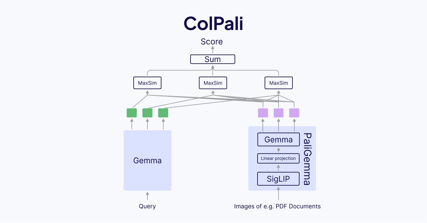
ColPali Model Architecture

ColPali was created in a similar way to ColBERT. What BERT is to ColBERT, PaliGemma is to ColPali. Essentially, instead of using BERT as the query and document encoder, ColPali uses the PaliGemma Vision LLM, which is separated into two parts for the query and document. Since queries will always be text-only, it uses Gemma (the language-only part of PaliGemma) as the query encoder and PaliGemma (the full vision model) as the vision encoder. Just like ColBERT, ColPali stores the pre-computed document vectors offline, and uses late interaction to compare to online embedded queries at runtime. ColPali has:

• ~3B parameters
• 128 embedding dimension size
• max 1024 patch size

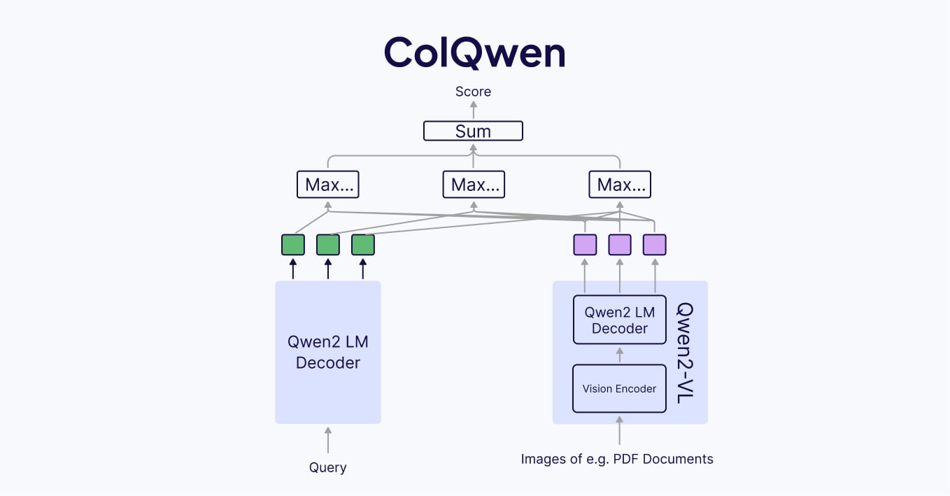
ColQwen Model Architecture

ColQwen is extremely similar to ColPali, with a different vision language model, Qwen2 Vision LLM, as the encoder. ColQwen uses Qwen2 LM as the query encoder and Qwen2-VL as the vision encoder. Whilst having a similar architecture to ColPali, the details are different due to using a completely different encoder model:

• ~2B parameters
• 128 embedding dimension
• max 768 patch size

Additionally, ColQwen’s vision language backbone model is licensed under a permissive apache2.0 license.

Advantages and Limitations of ColPali and ColQwen

The advantages of multimodal late interaction retrieval models like ColPali and ColQwen are that they allow for RAG applications without a complex preprocessing or chunking strategy for the PDF documents. Both text and images in PDF documents can be simply treated together as 'screenshots', which the vision models in ColPali and ColQwen can see and process. This also means figures in documents can be placed contextually with the text of the document, and these documents are processed similarly to how a human would read them.

But while ColPali and ColQwen both simplify the normally complex pipeline for PDF document processing, they also requires more resources to store all individual image patch embeddings, even with compression mechanisms, similar to ColBERT.

Use Cases of ColPali and ColQwen

Because of their multimodal capabilities ColPali and ColQwen are great for retrieval pipelines that process complex documents like PDFs, containing different components like text, images, graphs, tables, and formulas.

You can find a multimodal RAG over PDF documents code example with ColPali in Python in our recipes repository on GitHub.

Summary

This article discussed the late interaction mechanism and its retrieval models, such as ColBERT, ColPali, and ColQwen. In contrast to no-interaction models and full-interaction models, which are either effective or scalable, late interaction models are fast and effective retrieval models. That’s why they are a great fit for applications that require an effective and efficient retrieval process.

The added multi-modality in ColPali and ColQwen allows us to build RAG pipelines over complex documents, such as PDF files, by converting them into images. Although late interaction retrieval models require more memory because of the multi-vector embeddings, they also offer a richer contextual understanding of both text and image files. That’s why multimodal late interaction retrieval models are especially useful in multimodal rag pipelines for processing complex documents, such as PDF files.

If you want to start playing around with the discussed late interaction models, you can find code examples here:

• RAG code example with ColBERT in our documentation.
• Multimodal RAG over PDF documents code example with ColPali in Python in our recipes repository on GitHub.

FAQ

What’s the difference between ColBERT and dense vector methods?

The difference between ColBERT and dense vector methods is that these traditional dense methods pool token-wise embeddings into a single representation while ColBERT embeddings keep the token-wise representations in a multi-vector embedding. It would be inefficient to keep token-wise representations from traditional dense embedding models because they are not trained for this purpose, whereas multi-vector embedding models like ColBERT are. The benefit of keeping the token-wise representation is that it allows for a more detailed understanding of the semantic similarity between the query and the search results. Additionally, there’s no loss of context as embeddings remain at the token level.

What’s the difference between BERT vs. ColBERT?

The difference between BERT and ColBERT is that the offline computation of document embeddings allows ColBERT to be faster at run-time compared to BERT. BERT requires embedding queries and documents together in order to provide a comparison, whilst ColBERT has the document embeddings pre-computed and stored.

On a side note, ColBERT uses a fine-tuned version of BERT as encoders for both the query and the documents.

What’s the difference between ColBERT vs. ColBERTv2?

The difference between ColBERT and ColBERTv2 is the improved storage efficiency and higher retrieval effectiveness in the newer model. Any multi-vector model suffers from high storage costs due to the requirement of storing multiple vectors per document, which scales highly with the number of tokens in a document. ColBERTv2 alleviates the storage issues by heavily quantizing the token vector embeddings, and storing a subset of ‘nearby’ centroid vectors in higher precision. Combining the centroids with the quantized vectors gives a very good approximation to the true token embedding whilst minimizing the storage costs of each vector.

Additionally, ColBERTv2 gains strong retrieval performance over ColBERT by distilling knowledge from a larger, more impractically sized model (MiniLM), as well as by training the model to learn to distinguish between similar but incorrect documents and the correct documents for a given query.

What’s the difference between ColBERT vs. ColPali and ColQwen?

The difference between ColBERT vs. ColPali and ColQwen lies in the modalities these retrieval models are able to handle. Because ColBERT uses BERT, it is able to handle only text. In contrast, ColPali and ColQwen use VLMs and are therefore multimodal and can handle both text and images. While the search query for all models is a text input, the type of documents to search over is different between the models. ColBERT processes documents in text format, while ColPali and ColQwen process images, including PDF documents treated as images.

What’s the difference between ColPali vs. ColQwen?

The main difference between ColPali and ColQwen is that ColQwen uses the Qwen vision LM, whereas ColPali uses the PaliGemma VLM (and Gemma LM for embeddings). Additionally, the Qwen2 VLM has 1 billion parameters fewer than the PaliGemma VLM, making ColQwen a smaller model. ColQwen also has a smaller image patch size, which can result in lower storage and computational costs.

Resources

• ColBERT paper: https://arxiv.org/abs/2004.12832
• ColBERT v2 paper: https://arxiv.org/abs/2112.01488
• ColPali paper: https://arxiv.org/abs/2407.01449
• PaliGemma paper: https://arxiv.org/pdf/2407.07726

Ready to start building?

Check out the Quickstart tutorial, or build amazing apps with a free trial of Weaviate Cloud (WCD).

GitHub

Forum

Slack

X (Twitter)

Don't want to miss another blog post?

Sign up for our bi-weekly newsletter to stay updated!

By submitting, I agree to the Terms of Service and Privacy Policy.