
How to Reduce Memory Requirements by up to 90%+ using Product Quantization
- Product Quantization - how PQ reduces the memory requirements of running Weaviate
- Improving PQ with Rescoring - why compressing vectors decreases recall and how the rescoring trick can help reduce this
- Experimental results - QPS vs. recall, indexing times, and memory savings
- Benchmarking PQ - scripts for benchmarking PQ with your own data
What is Product Quantization (PQ)?
Product Quantization is a way to compress vectors, allowing users to save on memory requirements. To understand how product quantization (PQ) compression works, imagine every vector you want to store is a unique house address. This address allows you to precisely locate where someone lives including country, state, city, street number, and even down to the house number. The price you pay for this pin-point accuracy is that each address takes up more memory to store. Now, imagine instead of storing a unique address for each house we store just the city the house is located in. With this new representation, you can no longer precisely differentiate between houses that are all in the same city. The advantage however is that you require less memory to store the data in this new format. This is why PQ is a lossy algorithm; we lose information as a result of the compression - or in other words, you trade accuracy/recall for memory savings.
Want to further reduce memory usage at the price of recall? Zoom out further and represent each address instead with the state it’s located in. Require more recall at the price of increased memory? Zoom in and represent the address on a more accurate scale. This tunable balancing of memory usage vs. recall is what makes PQ a great way to improve the flexibility of Weaviate for different use cases and customers.

Similar to the analogy above, in PQ compression instead of storing the exact vector coordinates, we replace them in memory with a learned code that represents the general region in which the vector can be found. Now imagine you conduct this compression for millions or even billions of vectors and the memory savings can become quite significant. Using these PQ compressed vectors stored in RAM we now start our search from our root graph quickly conducting broad searches over PQ compressed vector representations to filter out the best nearest neighbor candidates in memory and then drill down by exploring these best candidates when needed.
If you’d like to dig deeper into the inner workings of PQ and how these compressed vector representations are calculated please refer to our previous blog here.
In this blog we cover how we can take this one step further, with 1.21 we introduced significant improvements to make PQ even more viable by reducing the recall price you pay in order to save on memory requirements. If you want to learn about these improvements and why using PQ should be a no-brainer now for most users, keep reading!
The problem with PQ
Our goal with the use of PQ is to reduce memory usage while maintaining a high quality of search - preferably the same search quality as when using uncompressed vectors. With the pure PQ implementation we had in v1.18 we paid a high recall/search quality price when the data was compressed at higher ratios.
To demonstrate this loss of recall due to compression we show a compressed vs. uncompressed graph below. These results compare the HNSW+PQ compressed implementation versus using HNSW with uncompressed vectors.
For our tests below, we use two different datasets: Sphere and DBPedia. The original Sphere dataset contains nearly 1 billion vectors of 768 dimensionality, however, in these initial experiments, we use a subset containing only 1 million vectors. We will revisit the entire dataset at the end of this post. DBPedia is a set of 1 million objects vectorized using the Ada002 vectorizer from OpenAI. These are both sizable and high-dimensional realistic datasets that could very well be used for real-world applications.
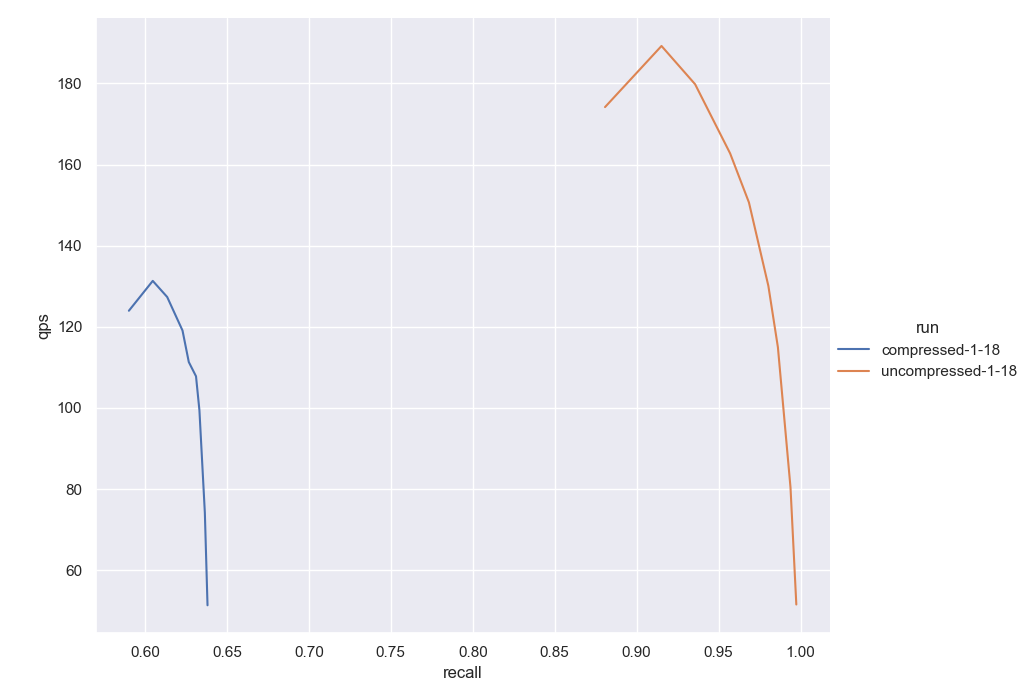 Fig. 1: The figure above shows results on a 1M subset of Sphere. The orange curve represents the results obtained with the uncompressed version. The blue curve shows the results of compressing using 6 dimensions per segment. This would achieve a 24:1 compression rate. Notice how the performance is comparable but the recall drops drastically.
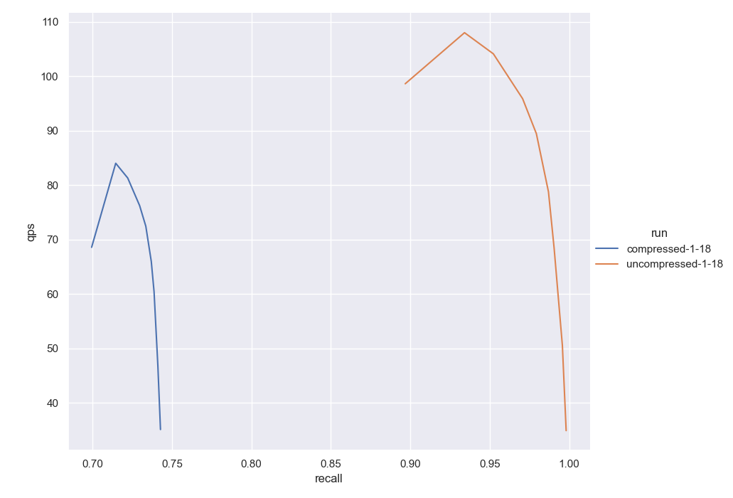 Fig. 2: The figure above shows results on the DBPedia dataset. The orange curve represents the results obtained with the uncompressed version. The blue curve shows the results of compressing using 6 dimensions per segment - compressing by a factor of 24x. Again, performance is preserved but the recall drops drastically.
A quick explanation for the dip in the graph at the left end. Those curves were obtained by querying the server right after indexing the data. After the indexing, it normally follows intense operations such as compactions or garbage collection cycles. After those operations finish, the full CPUs are again ready and there are no locks on the data. Notice how normally the second point in the curve is always smooth again.
Coming back to the main thread, this graph paints a pretty bleak picture! It seems inevitable that the more you compress the vectors, the more you will distort them and the further recall will drop. So how do we reduce this drop in recall while still achieving high compression ratios?🤔It starts with understanding: Why did the recall drop so drastically in the first place?
Improving recall with product quantization(PQ)
The reason for this reduction in recall, across both experiments, is that after compression you only have 1/24th the amount of information stored in the vectors - the vectors are only a fuzzy estimation of what they used to be. Originally, we had a continuous vector space. After compression, we only have a discrete/quantized vector space. This is because all the vectors are now encoded with approximate groups of regions rather than unique coordinates - refer to the diagram below for a better understanding of what we mean by “regions”.
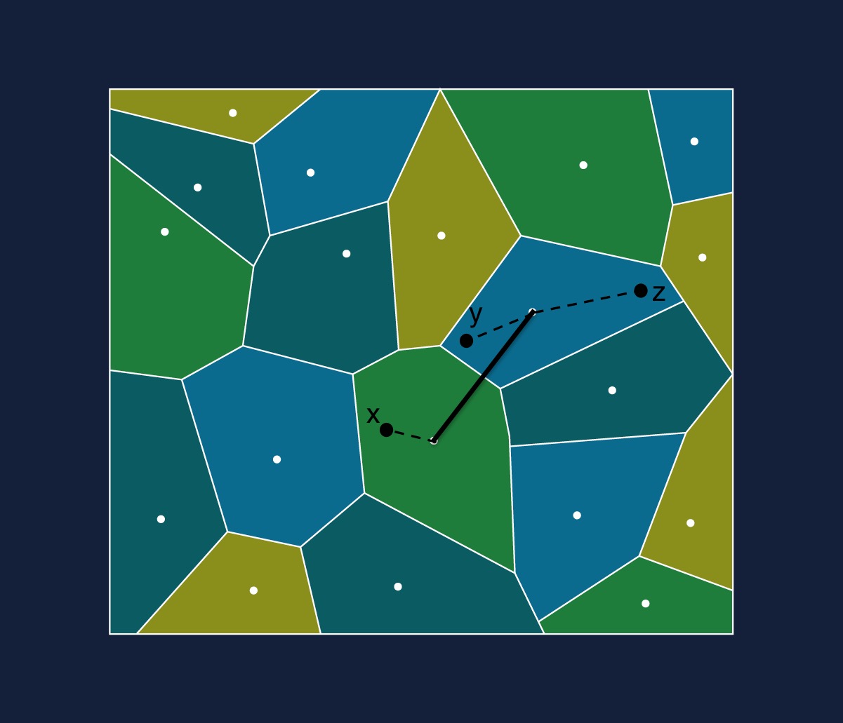 Fig. 3: Here all the vectors that lie inside a region will have the same code - the coordinates of the white dot in that region - this is shown using a dotted line from the vector to the centroid. This is what allows us to save space, but also reduces recall since the vectors within the regions become indistinguishable from each other.
If we have three vectors , and represented with the closest centroids to them shown in white above, and if we measure the distance between and compared to and and if these are equal, , then all we know about and is that they used to be close to each other prior to compression - we can’t calculate how close they were, additionally we can no longer calculate if is closer to or since we don’t have exact distances to compare. As a result, when the nearest neighbors algorithm calculates the distances between the query and compressed vectors it might not always identify the most relevant vectors to return to the user.
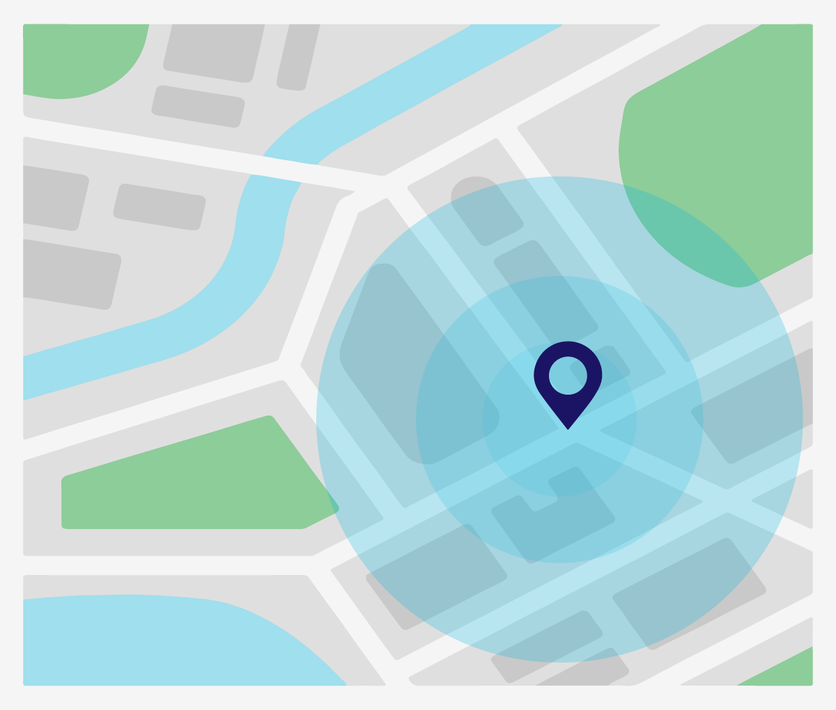
Imagine you were invited to a birthday party in another country and instead of being given the full address you were only told the city where the party is! You might be able to roughly search up and travel to the right city in the country but finding the party within the city would be impossible. Try as hard as you might, you’re not going to be showing up to that party! 😅
Similarly, we can use our compressed vectors to perform a rough search to identify objects that might be relevant or not and land us in the right “city” in vector space, but we still need a way to perform a finer search as we get closer to our target query. This finer search is made possible by the fact that we actually store the full un-compressed representation of the vectors on disk and can read them into working memory when/if required! Aha! A solution presents itself!
Putting all the pieces together let's say you get a query from the user, this gets converted into a vector and we start to perform a rough search comparing the query vector to compressed object vectors, to identify which objects are relevant (close enough) - if an object is found to be relevant we put it in the relevant bucket otherwise we throw it out. Once we have our bucket of relevant vectors we then fetch their uncompressed representations from disk into memory and use this to rescore the vectors in our bucket from closest to furthest to our query vector!
Thus, this rough search followed by a finer search and rescoring allows us to reduce memory usage while still maintaining recall. Seems perfect no, why wouldn’t we always do this!? We get to have our cake and eat it too! Not quite!
The only way recall would be lost when employing this new strategy is if the rough search over compressed vectors fails to identify some relevant vectors and these candidates never make it into the bucket for the finer rescoring search phase. Let's consider some implementation details that can help avoid this potential failure mode.
The devil is in the details
Before digging deeper, let's think about the final goal we’re trying to solve.
We use PQ because we want to save on memory. If we only have a few hundred thousand vectors we wouldn’t consider using PQ - as memory usage would be negligible. On the other hand, if we need to store billions of vectors then PQ becomes critically important - without it, we might not even be able to store all of our data. The problem that arises, however, is that a billion object vector space is quite crowded and since vectors are represented using regions/clusters with PQ encoding you’re likely to find more vectors in any given region - each of which will have the same coded representation. Refer to the diagram below for an intuitive representation of this “crowding” effect.
| 100K Vector Space | 1B Vector Space |
|---|---|
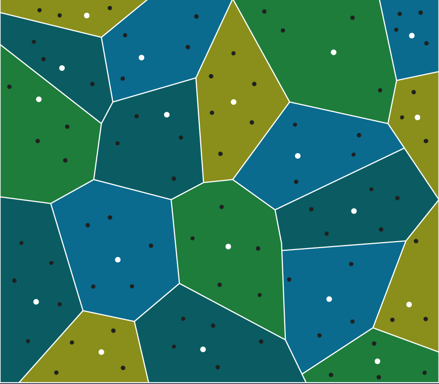 |  |
Fig. 4: Notice how the vector space representation on the bottom is a lot more crowded, due to there being more vectors(represented as black dots). Each of the vectors in a region will have the coordinates of the centroid for the region(represented as white dots). This means that all vectors in a region after compression become indistinguishable. Note that in PQ this is not exactly what happens but this does give us a good intuition of how the distortion is more noticeable when we have more vectors
So the conundrum is this: the more data you have the more you will want to use PQ to compress it, but on the other hand, you’ll have more crowding which will distort data more and potentially reduce recall.
To address this we explored two implementation strategies for our rescoring solution explained in the section above:
-
Strategy 1: Conducting the rough search and finer search together. This is done by rescoring the distances during the search process.
-
Strategy 2: Conducting the finer search after the rough search has concluded. This is done by only rescoring after we have obtained the final bucket of relevant objects.
Strategy 1 gave us better recall because we got to determine object relevance using exact distances prior to putting them in our bucket - but performance suffered since we’re doing more disk reads to accomplish this.
Strategy 2 ensured better performance - since we would do one disk read at the conclusion of the rough search, but recall suffered due to relevant objects not being included in our bucket during the rough search phase.
In the PQ implementation of Weaviate v1.21, we have decided to adopt Strategy 2. This was because we found that its low recall problem could be addressed by tuning search parameters - or in other words by making our bucket of relevant objects larger. Simply stated, if we fear losing relevant objects during the rough search phase, due to PQ distortion, then storing more of them will reduce this. In our experiments, we found that using this technique we could achieve the same recall as Strategy 1 at lower latencies! Voila 🎉, we have a winner!
🔬Experiment Results
Below we show experiments comparing the new in improved v1.21 PQ. Our experiments focus on recall, latency, indexing time, and memory savings.
QPS vs Recall Experiments:
First, we show the comparison of the results of our old implementation (without rescoring nor the last optimizations) with the last implementation (v1.21). Our first point of comparison is in terms of performance (measured in QPS) against quality (measured in recall)
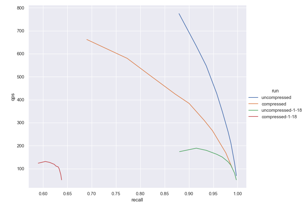 Fig. 5: The image above shows the results in the Sphere dataset. We have included the four curves now. The results labeled as
 compressed/uncompressed-1-18 refer to the old implementation while the other two represent the new 1.21 results achieved using rescoring and better code optimization.
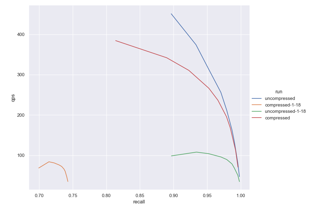 Fig. 6: The image above shows the results in the DBPedia dataset. We have included the four curves now. The results labeled as
 compressed/uncompressed-1-18 refer to the old implementation while the other two represent the new results achieved using rescoring and better code optimization.
As you might notice, both datasets follow similar profiles. There is a huge difference also between the uncompressed cases. This is because with version 1.19 of Weaviate we have introduced gRPC support and querying is much faster overall. We have also included SIMD optimizations for the distance calculations for the uncompressed case. Unfortunately, those SIMD optimizations cannot be used for our current compressed version - but those are details for another time!
That being said, notice how the recall is no longer lower for the compressed version. To stress this out, if we compare the orange curve (compressed using v1.18) to the green curve (uncompressed using v1.18) we can notice the shifting to the left in the recall axis. Notice also that this shift is not small. Now comparing the red curve (compressed using v1.21) to the blue curve (uncompressed using v1.21) the two curves are very close together in terms of QPS and recall.
Indexing Time Results
Previously we were also experiencing longer indexing times when using PQ. The main bottleneck was distance calculations between already compressed vectors in the implementation of our pruning heuristic. To help with this issue, we have introduced a special lookup table with distances between compressed segments. This acts similarly to the lookup table centered at each query, but unlike the former which is more volatile, it will reside in memory during the full indexing process.
Due to these improvements we now see improved indexing times, please refer to the profiles below. The table below shows the indexing times measured for all cases. Notice how the v1.21 needs approximately the same time to index the data for both, compressed and uncompressed cases. This was not the case in earlier v1.18 and was only possible with the introduction of the global lookup table.
| Indexing Time | Version | Compressed (hours) | Uncompressed (hours) |
|---|---|---|---|
| Sphere | 1.18 | 1:01:19 | 0:30:03 |
1.21 | 0:26:42 | 0:30:03 | |
| DBPedia | 1.18 | 1:25:00 | 0:51:49 |
1.21 | 0:51:34 | 0:52:44 |
Tab. 1: Indexing time improvements between v1.18 and v1.21.
Memory savings
Last but not least, our goal with compression is to save memory. We have seen two implementations indexing the data at the same speed and serving queries at very similar performance/quality profiles. The main benefit here is the memory footprint. The table below shows the heap memory used for both cases. We keep it simple this time and only show our last version (1.21) since the memory footprint is similar to the older version 1.18.
| Memory footprint (MB) | Compressed (hours) | Uncompressed (hours) |
|---|---|---|
| Sphere | 725 (15%) | 5014 |
| DBPedia | 900 (14%) | 6333 |
Tab. 2: Compression ratios of ~6.6x.
Notice how using the compressed version we would barely need 15% of the memory we would need under uncompressed settings.
To close the results up, we have also indexed the full Sphere dataset (nearly 1 billion vectors) with and without compression. The full dataset without compression needed nearly 2.7 Terabytes of memory while the compressed version only required 0.7 Terabytes which is again, a huge saving in terms of memory and costs.
📈Benchmarking PQ with your own data
If you're trying to finetune HNSW and PQ parameters on your own data to optimally balance recall, latency, and memory footprint you might want to replicate these experiments yourself. While doing so, please pay special attention to the segments parameter. We have obtained the best results using segments of length 6 in our experiments with both: Sphere and OpenAI embeddings.
We have included some very useful tools in our chaos pipelines. To easily run these tests (or any test using your own data) you would need the data to be in hdf5 format with the same specifications as described in the ANN Benchmarks. You could index your data using the run.py script under the ann-benchmarks folder. It admits several parameters that you could explore but in our runs, we use the following commands:
To run uncompressed (PQ disabled):
python3 run.py -v sphere-1M-meta-dpr.hdf5 -d dot -m 32 -l run=uncompressed
Notice the -d parameter for the distance and -m for the maximumConnections.
To run compressed (PQ enabled):
python3 run.py -v sphere-1M-meta-dpr.hdf5 -d dot -m 32 --dim-to-segment-ratio 6 -c -l run=compressed
Notice the -c flag to set compression on and the –dim-to-segment-ratio to specify how long you want your segments to be. In this case, we are using 6 dimensions per segment.
Once you run the script, you will see the different metrics in your terminal at the end of the run. Pay special attention to the qps, recall and heap_mb (heap size in MB). You will also have the results in JSON format under a repository named results in the same path as the script. Next, you can also run the visualize.py script to produce the same graphs we show in this post. Your graphs will be available in the same path as the script as output.png. To differentiate between your different runs, use a different value for the run parameter when using the run.py script. The label you use for the run will be used for the curve generated after running the visualize.py script.
Conclusions
In this post, we explore the details behind how we improved the implementation of PQ in Weaviate to reduce the loss of recall by introducing a rescoring trick that reads in uncompressed vectors from disk and recalculates exact distances during the search process.
As a result of rescoring when using PQ in Weaviate the trade-off between memory savings and recall is great. For this reason, most applications and users of Weaviate can now use PQ as the default. To further improve your results when using PQ we suggest you benchmark with your own data to balance compression ratios against reduction in recall. Happy compressing!🚀
Ready to start building?
Check out the Quickstart tutorial, or build amazing apps with a free trial of Weaviate Cloud (WCD).
Don't want to miss another blog post?
Sign up for our bi-weekly newsletter to stay updated!
By submitting, I agree to the Terms of Service and Privacy Policy.